Integration Multi-Model to Evaluate the Impact of Surface Water Quality on City Sustainability: A Case from Maanshan City in China

Abstract

Water pollution is a worldwide problem that needs to be solved urgently and has a significant impact on the efficiency of sustainable cities. The evaluation of water pollution is a Multiple Criteria Decision-Making (MCDM) problem and using a MCDM model can help control water pollution and protect human health. However, different evaluation methods may obtain different results. How to effectively coordinate them to obtain a consensus result is the main aim of this work. The purpose of this article is to develop an ensemble learning evaluation method based on the concept of water quality to help policy-makers better evaluate surface water quality. A valid application is conducted to illustrate the use of the model for the surface water quality evaluation problem, thus demonstrating the effectiveness and feasibility of the proposed model.

1. Introduction

It has long been recognized that water pollution has negative impacts on human health and ecosystems [1]. Regarding human health, the most immediate and most severe impact is the lack of improved sanitation, associated with the lack of safe drinking water, which currently affects more than one third of the world’s population [2]. Water pollution is caused by industrial and anthropogenic activities, such as industrial accidents [3,4], urbanization [5,6] and natural phenomena like soil erosion [7,8]. Additional threats include, for example, exposure to pathogens or chemical toxicants via the food chain (e.g., as a result of irrigating plants with contaminated water and of the bioaccumulation of toxic chemicals by aquatic organisms, including seafood and fish) or during recreation (e.g., swimming in contaminated surface water) [9,10]. Serious water pollutants will cause different degrees of loss to industry. Therefore, the prevention and control of water pollution is a top priority in all of life and industry [11].

To effectively solve the problem of water pollution at several spatial scales, water quality modeling is of utmost relevance for evaluation. A Multiple Criteria Decision-Making (MCDM) model is developed in this case for evaluating water quality. The measurement of water quality is one way of comparing degrees of water pollution [12]. There have been several works devoted to evaluating water pollution. For example, Reference [13] used MCDM techniques to present different aspects of water pollution control and reported the results of a case study for developing a master plan for water resources pollution control in Isfahan Province in Iran. Reference [14] reported the application of fuzzy MCDM for ranking different types of industries based on water pollution potential in the State of Gujarat, India. Fuzzy analytic hierarchy process, as one of the most versatile MCDM methods, was used for managerial decision-making in complex surface water pollution situations with multiple and varied measures [15]. An alternative evaluation index system was developed to establish the priorities of a range of water pollution alternatives using MCDM techniques [16].

However, existing methods may obtain different evaluation results in the same case, so it is difficult for policy-makers to decide which method to employ. In this circumstance, ensemble vote, as a kernel of ensemble learning, can represent a good assistant to solve the multi-MCDM model problem [17]. Ensemble learning can not only solve the problem of evaluation result non-conformity in water pollution, but also solve water pollution environmental management issues.

MCDM methods have been applied to a wide range of application areas. For instance, the Technique for Order Preference by Similarity to an Ideal Solution (TOPSIS) is used primarily in the manufacturing, industry, and government sectors. Analytic Hierarchy Process (AHP) is used for evaluating weight derivation and it is still the most popular method despite some criticism in recent years [18]. Meanwhile, the hybrid learning style was applied in research suggesting that an integrated TOPSIS model could be used to solve the truck selection problem of a land transportation company [19]. A novel conjunctive MCDM approach that combines AHP and TOPSIS was used to develop an innovation evaluation system for location selection [20]. Similarly, a hybrid ensemble approach was used in a suppliers’ selection problem, applying ensemble methods to obtain a better predictive performance than that achieved by an individual algorithm [21]. A novel hybrid ensemble learning paradigm integrating ensemble empirical mode decomposition was proposed for nuclear energy consumption forecasting, and empirical results demonstrated that the ensemble learning paradigm could outperform some forecasting models in both prediction and directional forecasting [22]. Furthermore, water quality is of great importance to our daily lives and is forecasted by using a multi-task multi-view learning method to blend multiple datasets from different domains [23]. The results of this evaluation are inconsistent between different models even under the same cases. Therefore, the proposed ensemble learning paradigm is used for the evaluation of water quality in this paper.

To address the aforementioned concerns, this paper proposes hybrid ensemble learning for a data-mining evaluation framework, which combines the TOPSIS [24], Grey Relational Analysis (GRA) [25], AHP [26], and Takagi-Sugeno (TS) fuzzy neural network [27,28].

The main objective of this work is to select and combine some algorithms of optimum configuration for an integration of multiple MCDM models in a framework based on multi-criteria evaluation. The main motivation is to evaluate water quality in six sites. Related work is discussed in Section 2. Section 3 proposes the frame and the methodology. The results and discussion are given in Section 4. The conclusions of this work are summarized in Section 5.

2. Related Work

Generally, most of the criteria required in MCDM cannot be evaluated accurately, since it is impossible to obtain precise data concerning the assessment of the decision makers. Moreover, some of the criteria are only evaluated subjectively, leading to incorrect results [29]. MCDM is widely used in many evaluation cases, and it is used in the evaluation of water quality in our research. Therefore, we focus on comparing water quality in different sites to compare the water pollution degree of different sites according to the required water criteria [30]. Water quality evaluation refers to the understanding of water quality conditions, which is a complex problem involving multiple disciplines. Many countries established relevant standards for different types of water systems. Water quality standards for surface waters are established by foundation of the water quality-based pollution control schemes under the Clean Water Act (CWA) in the USA [31]. Meanwhile, China promulgated the surface water quality standards (GB3838-2002) for the surface water quality evaluation of rivers and lakes in 2002 [32]. Evaluation theory and evaluation methods have enjoyed great developments in the recent years. For instance, the index evaluation method [33], fuzzy evaluation method [34], Grey theory evaluation method [35], and neural network evaluation method have been put forth by different researchers [36].

As an active research area, several evaluation methods have been proposed. For example, TOPSIS is used to evaluate the nature of green supplier selection. This is a complex multi-criteria problem, including both quantitative and qualitative factors, and there may be conflicts and uncertainness. The identified components are integrated into a novel hybrid fuzzy MCDM model that combines the TOPSIS with the Analytical Network Process [37]. Meanwhile, the hybrid learning style is applied, and some research has suggested integrating the TOPSIS model to help the industrial practitioners with performance evaluation in a fuzzy environment [38]. Similarly, a novel conjunctive MCDM approach that combines AHP and TOPSIS order was employed to develop an innovation support system that considers the interdependence of higher education institutes to comprehensively evaluate their innovation performance [39]. Another study presented the application of multi-criteria evaluation in the selection of an optimal allocation for an air quality model [40], which was developed to support managers in exploring the strengths and weaknesses of each alternative. This approach identifies a preferred result based on the integration of Bayesian networks and fuzzy logic to rank and evaluate suppliers [41].

MCDM and integrating machine learning algorithms have been developed in recent years, including some hybrid methodology techniques that have effectively been used to conduct multi-attribute inventory analyses. For instance, naive Bayes, Bayesian network, artificial neural network (ANN), and support vector machine (SVM) algorithms [42], they have successfully dealt with inventory classification problems. Financial risk prediction is used by MCDM methods (e.g., TOPSIS) to develop a two-step approach to evaluate classification algorithms, and results show that linear logistics, Bayesian network, and ensemble methods are the top-three classifiers [43]. In the assessment of machine learning algorithms, selecting the appropriate classifier from the list of available candidates is a time-consuming and challenging task. Therefore, an accurate MCDM methodology evaluates and ranks classifiers based on experience, allowing end-users or experts to select the top-ranked classifier for their applications to learn and build classification models for their specific purposes [44].

3. Methods

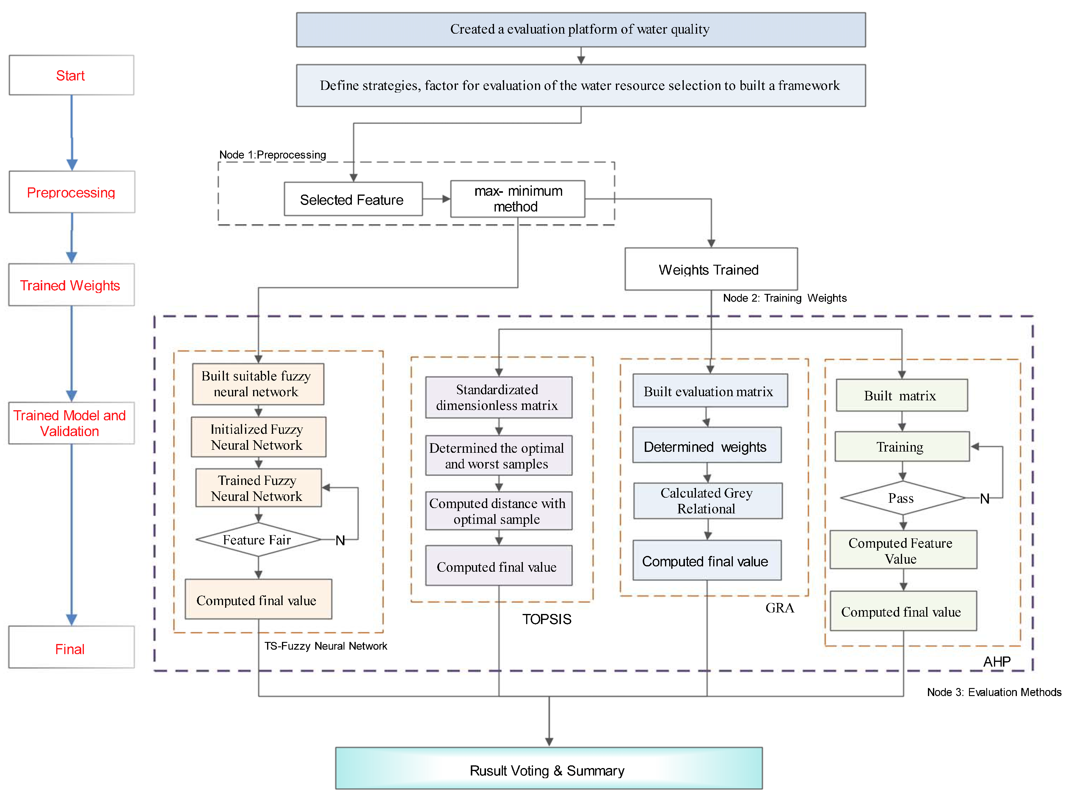
To demonstrate the above concerns, we propose a hybrid ensemble multi-model for a data-mining evaluation framework combining GRA, TS Fuzzy Neural Network, TOPSIS, and AHP, as shown in Figure 1. We know from Figure 1 that our framework consists of other key phases, including indicator preprocessing, a weights model, and an evaluation training model. In this work, the main contribution is shown in node 3, which have solved different results from multiple model evaluation, that is to say, a consistent result is obtained by ensemble vote. We describe the phases in detail in the following sections.

3.1. Ensemble Learning Approach

Ensemble learning is a learning task by building and combining multiple learners [45]. There are two main advantages in this method. One is multiple training machines which can achieve the same performance if the learning task is large from the perspective of statistics. Also, this multiple model would reduce risk, because it may not lead to the wrong selection compared to a single model. The other one is learning algorithms, which tend to fall into the local minimum, and lead to poor generalization performance from a computational perspective. Meanwhile, a combination of multiple models and learning algorithms can reduce the risk of falling into a bad local minimum. In addition, some learning tasks may not satisfy the current hypothesis learning algorithm, and a single model would definitely be invalid in this case. By combining with multiple models, the corresponding hypothesis space has a better expanded learning better. Therefore, the ensemble learning is often adopted to improve the overall accuracy of regression and classification methods [46]. We used the ensemble vote integration results of a multi-MCDM model evaluation to obtain a more accurate result. The given ensemble includes T model $h_1,h_2,\dots ,h_T$, where the $h_t$ output is $h_t\left(x\right)$ in training set x. The voting is involved in the testing stage, when the independent prediction is combined to predict an invisible instance. Some popular methods of voting include equal voting, weighted voting, and naive Bayesian voting. This paper employs the weighted voting method, in which the weights of each models are the different, as shown in Equation (1).

$$H\left(x\right)=\frac{1}{T}\sum _{t=1}^T{\omega }_t{h}_t\left(x\right)$$

(1)

where $h_t\left(x\right)$ is a single training model result, $\omega$ is the model result weights, $H\left(x\right)$ is the ensemble value of each model’s result, and T is the count.

3.2. Evaluation Based on TS Fuzzy Neural Network System

ZadehLA, an American cybernetics expert at the University of California, pioneered the concept of fuzzy sets in 1965 [47]. Fuzzy theory has captured the characteristics of the ambiguity of human thinking and can thus be used to solve conventional problems.

TS fuzzy systems have a very strong self-adaptive ability, which can automatically update and modify the membership function of fuzzy subsets. Therefore, the error of a model is modified slowly in the running process, and the result is relatively better. A TS fuzzy system has a set of “if-then” rules to be defined. Concerning the rules for the $R^{\prime }$, the fuzzy reasoning is as follows:

$$R^i:\mathrm{If}{x}_1\mathrm{is}{A}_1^i,x_2\mathrm{is}{A}_2^i,\dots ,x_n\mathrm{is}{A}_n^i,\mathrm{then}{y}_i=p_0^i+p_1^i{x}_1+\dots +p_n^i{x}_n,$$

(2)

where $i=1,2,3,\dots ,m$, $j=1,2,3,\dots ,n$, and so on, hereinafter; $A_j^i$ is the fuzzy sets for the fuzzy systems; $p_j^i$ is the parameters of the fuzzy system; and $y_i$ is the output according to the fuzzy rules. If the input part (i.e., “if”) is fuzzy, then the output part (i.e., “then”) is determined.

For input value $\mathbf{x}=[x_1,x_2,\dots ,x_n]$, the membership of each input variable is $x_j$ according to fuzzy rules is:

$$\mu A_j^i=e^{-\frac{{(x_j-c_j^i)}^2}{b_j^i}},i=1,2,\dots ,m,j=1,2,\dots ,n,$$

(3)

where $c_j^i$, $b_j^i$ represent the membership function center and width, respectively; n is the input parameters; m is the number of fuzzy subsets.

The calculation of the fuzzy degree of membership, fuzzy operator for the multiplication operator is as follows:

$$w^i=\mu A_j^i\left(x_1\right)\times \mu A_j^i\left(x_2\right)\times \dots \times \mu A_j^i\left(x_n\right).$$

(4)

According to the fuzzy results, to compute the model output value $y_i$:

$$y^i=\frac{{\sum }_{i=1}^m{w}^i(p_0^i+p_1^i{x}_1+\dots +p_n^i{x}_n)}{{\sum }_{i=1}^m{w}^i}.$$

(5)

However, model is lack of ability to learn in the application of the fuzzy comprehensive evaluation, due to complex optimization of the model parameters. The ANNs have self-learning, ability of self-organization and self-adaptation. If the combining them, they can effectively play their respective advantages.

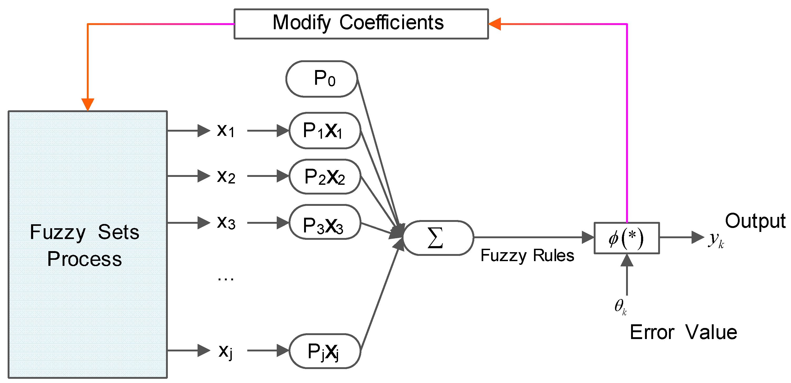
To obtain the evaluation result, the back-propagation (BP) neural network combined with the TS fuzzy system for training was employed. Figure 2 displays a neural network training procedure.

There is also a ${\theta }_k$ (or threshold $b_k=-{\theta }_k$). The above can be expressed mathematically:

$$u_k=\sum _{j=1}^n{w}_{kj}{x}_j,v_k=u_k-{\theta }_k,y_k=\varphi \left(v_k\right),$$

(6)

where $x_1,x_2,x_3,\dots ,x_n,$ are input signals; $w_{k1},w_{k2},w_{k3},\dots ,w_{kp},$ are the weights of neurons k; $u_k$ is a linear combination; ${\theta }_k$ is a threshold; $\varphi (\ast )$ is the activation function; and $y_k$ is the output of neurons k.

The TS Fuzzy Neural Network is divided into the input layer, the fuzzy classification layer, fuzzy programming to calculate the layer, and output layer. The input layer relates to the input vector $x_i$, which is the same as the number of nodes and the dimensions of the input vector. The fuzzy classification layer uses the fuzzy degree of the membership function of input values to obtain the fuzzy membership value. The layers of fuzzy rules are based on the fuzzy multiplication formula. The output layer uses this formula to calculate the output of the fuzzy neural network. The learning algorithm of the fuzzy neural network is as follows.

(1)

The error computing

$$e=\frac{1}{2}{(y_d-y_c)}^2,$$

(7)

where $y_d$ is the network expectation output; $y_c$ is the actual output of the network; e is the actual output of the error.

(2)

The modified coefficient

$$p_j^i\left(k\right)=p_j^i(k-1)-\alpha \frac{\partial e}{\partial c_i^j},$$

(8)

$$\frac{\partial e}{\partial p_j^i}=\frac{{(y_d-y_e)}^2{w}^i}{{\sum }_{i=1}^m{w}^i}{x}_j,$$

(9)

where $p_j^i\left(k\right)$ is the coefficient of the neural network; $\alpha$ is the network learning rate; $x_y$ is the network input parameters; and $w^i$ is the product of the degree of membership of input parameters.

(3)

The modification parameter

$$c_j^i\left(k\right)=c_j^i(k-1)-\beta \frac{\partial e}{\partial c_i^j},$$

(10)

$$b_j^i\left(k\right)=b_j^i(k-1)-\beta \frac{\partial e}{\partial b_i^j},$$

(11)

where $c_j^i$, $b_j^i$ represent the membership function center and width, respectively.

3.3. Evaluation Based on TOPSIS

TOPSIS was first proposed by Hwang and Yoon in 1981 and developed by Chen and Hwang in 1992 [39]. The TOPSIS model was used to evaluate the characteristics of the comprehensive evaluation index system of water quality and the purpose of evaluation in this paper. The basic idea of the TOPSIS method is to calculate the distance between the best scheme and the worst scheme in the continuous time series of samples and use the relative degree of the ideal solution as the standard of comprehensive evaluation. The TOPSIS method is detects the evaluation object and the optimal solution, as well as the worst solution of the distance to sort. It is best when the evaluation object is closest to the optimal solution and as far away as possible from the worst solution, otherwise it is will not be optimal. Firstly, we standardized the original data sets. Then $R={\left(r_{ij}\right)}_{m\times n}$ was employed as the for normalized dimensionless data matrix, where $r_{ij}=\frac{x_{ij}}{\sqrt{{\sum }_{i=1}^n{x}_{ij}^2}},i=1,2,\dots ,m;j=1,2,\dots ,n$.

Secondly, we determined the positive ideal and negative ideal solutions. The best and worst values are respectively represented by $Y^{+}$ and $Y^{-}$. Then:

$$Y^{+}=\left\{\left(ma{x}_i{r}_{ij}\right|j\le n)\right\}=\{y_1^{+},y_2^{+},\dots ,y_n^{+}\},Y^{-}=\left\{\left(mi{n}_i{r}_{ij}\right|j\le n)\right\}=\{(y_1^{-},y_2^{-},\dots ,y_n^{-}\}.$$

(12)

Thirdly, we determined the relative closeness to the ideal solution. The relative closeness $C_i$ to the ideal solution can be expressed as follows:

$$C_i=\frac{D_i^{-}}{D_i^{+}+D_i^{-}},$$

(13)

where $D_i^{+}$ and $D_i^{-}$ are the separation of each alternative from the positive ideal solution and the negative ideal solution, respectively. Each is $D_i^{+}=\sqrt{{\sum }_{j=1}^n{(r_{ij}-y_j^{+})}^2},D_i^{-}=\sqrt{{\sum }_{j=1}^n{(r_{ij}-y_j^{-})}^2},i=1,2,\dots ,m$. The larger the $C_i$, the closer the sample is to the optimal sample point.

Fourth, in this paper, the fuse neural network and entropy method was used to determine the weights of the indicators. The main idea can be summarized by the Reference [24].

3.4. Evaluation Based on Grey Relational Analysis

The Grey system theory has been widely applied in various fields [25], and has been proven to be useful in dealing with information on poverty, incompleteness, and uncertainty. We used GRA to evaluate water quality. Firstly, we determined the evaluation matrix, then determined each indicator’s weights, as shown in Section 3.3. We then calculated the Grey relational coefficient:

$$\xi (x_{0j},x_{ij})=\frac{min{\Delta }_{ij}+\rho max{\Delta }_{ij}}{{\Delta }_{ij}+\rho min{\Delta }_{ij}},$$

(14)

where ${\Delta }_{ij}=\parallel x_{0j}-x_{ij}\parallel$ and ${\xi }_i(x_{0j},x_{ij})$ are the Grey relational coefficients between $x_{ij}$ and $x_{0j}$; $\rho$ is the distinguishing coefficient, $\rho \in [0,1]$. Finally, the Grey weighting relational was calculated,

$$r_{X_0,X_i}=\sum _j^n{w}_j\xi (x_{0j},x_{ij}),$$

(15)

where w is the weight of attribute j; while $r_{X_0,X_i}$ is the Grey relational grade between $X_i$ and $X_0$, which represents the level of correlation between the reference sequence and the comparability sequence.

3.5. Evaluation Based on AHP

AHP was put forth for operations research by Professor Saaty at the University of Pittsburgh in the 1970s [48]. The main indicators of this method reflect the nature of complicated decision-making problems. This process conducts an in-depth analysis of the influencing factors and their relationship with the base station. It also involves less quantitative information to make the decision-making process of mathematical thinking, for the multi-objective and multi-criteria or non-structure decision-making method of simple and complex decision-making problem. It is difficult to completely apply a quantitative decision-making model or method to a complex system.

AHP can be succinctly summarized for water quality modeling as follows: structuring the decision hierarchy of interrelated decision elements, collecting input data by pairwise comparisons of decision elements, evaluating the consistency of managerial judgements, and applying the eigen-vector method to compute relative weights.

Concerning the details of the process reported in the literature [49,50], the main difference that arises is establishment of the matrix. We determined the matrix, in accordance with the theory of scale relation and the relationships between indicators, as shown in

Table 1. Saaty’ s fundamental scale.

Intensity of Importance	Definition
1	Equal importance/preference
3	Moderate importance/preference
5	Strong importance/preference
7	Very strong or demonstrated importance/preference
2, 4, 6, 8	In between these two adjacent levels
9	Extreme importance/preference

. Similarly, we aimed to overcome the difficulty and discrimination of only expert scoring using this scale.

4. Case Study

The numerical experiment was performed with surface water quality data. The MCDM method was particularly pragmatic for visualizing the structure of complex causality. MCDM is a comprehensive approach to establishing and analyzing structural models that contain causal relationships among complex factors. It can clearly reveal the standard causality when measuring a problem. MCDM is a good technique for evaluating problems, and the relationship of systems is generally given by crisp values in building a structural model, as shown in node 3 of Figure 1.

4.1. Indicator Description and Data Preprocess

An environmental system is a complex system; therefore, water quality evaluation must also be a result of a multi-factor interaction. The impact of different factors on the degree of pollution varies, and that which has the greatest impact on the role of water pollution is known as the “main factor”. We thus needed to collect data of different action factors, analyze the data, and introduce the quantification index to evaluate the influence degree. According to this quantitative index, we could determine the water pollution degree shadow size. Therefore, based on the relevant water science data, we identified several factors that have a significant impact on water quality.

The relevant indicators surface water quality standard (i.e., GB3095-2002 standard [51]) from Ministry of Environmental Protection of China, combined with indicator selection for water quality. The final selection indicators were: $DissolvedOxygen\left(F_1\right)$, $BO{D}_5\left(F_2\right)$, $Manganate\left(F_3\right)$, $Ammonium\left(F_4\right)$, $NitriteNitrogen\left(F_5\right)$, $VolatilePhenol\left(F_6\right)$, $Cyanide\left(F_7\right)$, $TotalMercury\left(F_8\right)$, $TotalArsenic\left(F_9\right)$, and $HexavalentChromium\left(F_{10}\right)$. The standards are shown in

Table 2. National environmental quality standards for surface water (partial) (/mg·L ${}^{-1}$).

Level	${\mathit{F}}_1$	${\mathit{F}}_2$	${\mathit{F}}_3$	${\mathit{F}}_4$	${\mathit{F}}_5$	${\mathit{F}}_6$	${\mathit{F}}_7$	${\mathit{F}}_8$	${\mathit{F}}_9$	${\mathit{F}}_{10}$
1	7	2.8	2	0.015	0.06	0.002	0.005	5	0.05	0.01
2	6	3	4	0.02	0.1	0.002	0.05	5	0.05	0.05
3	5	4	6	0.02	0.15	0.005	0.2	10	0.05	0.05
4	3	6	8	0.2	1	0.01	0.2	100	0.1	0.05
5	2	10	10	0.2	1	0.1	0.2	100	0.1	0.1

, in which is Level 1 is best, Level 5 is worst.

Ten indicators were chosen to be measured for the determination of the best water quality. However, positive and negative values represent different meanings. For instance, $DissolvedOxygen$ is a positive indicator, while $BO{D}_5$ is a negative indicator. Therefore, we choose Equations (16) and (17) to normalize the positive and negative values. Data preprocessing was necessary and completed using two methods. The first was the max-minimum method that is used to train the weights, and the second was the standard method that is used to calculate the comprehensive score [52].

Positive indicators:

$$x_{ij}=\frac{u_{ij}-min\left(u_{ij}\right)}{max\left(u_{ij}\right)-min\left(u_{ij}\right)}$$

(16)

Negative indicators:

$$x_{ij}=\frac{max\left(u_{ij}\right)-u_{ij}}{max\left(u_{ij}\right)-min\left(u_{ij}\right)}$$

(17)

where $u_{ij}$ represents the original data, $x_{ij}$ represents the data after normalization.

4.2. Study Area

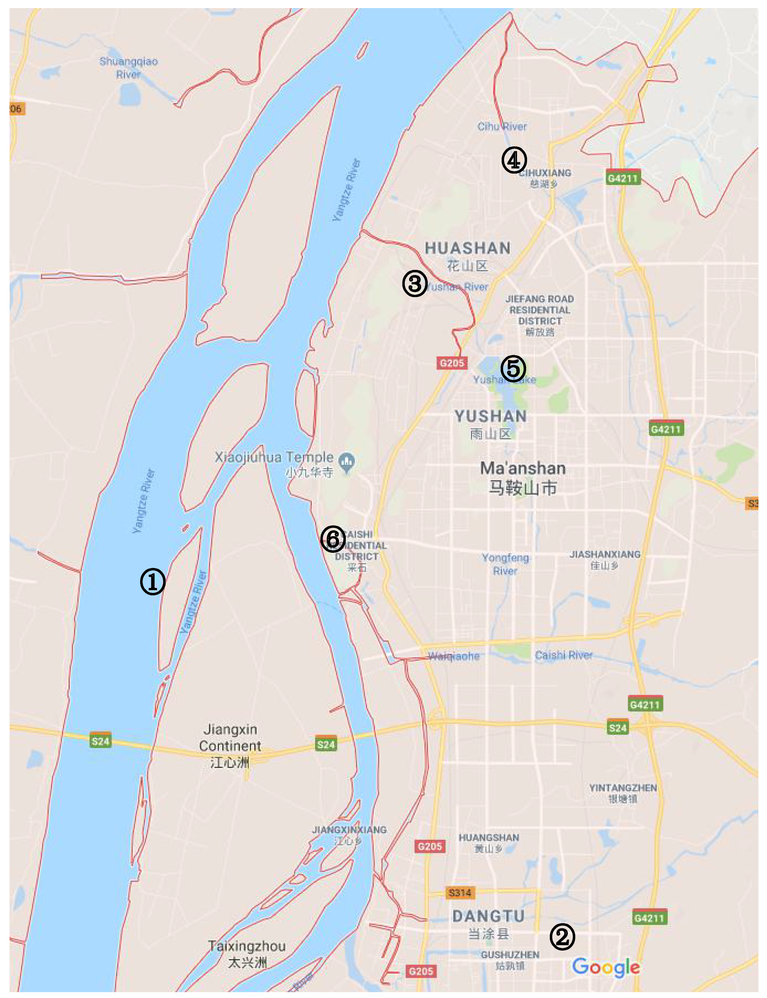
Ma’anshan, also colloquially written as Maanshan, is a prefecture-level city in the eastern part of Anhui province in Eastern China. It also is an industrial city stretching across the Yangtze River. Maanshan’s rivers mainly include the Ma’anshan Reach of the Yangtze River, Quarry River, Yushan River, Cihu River, Yushan Lake, and Suoxi River, corresponding to sites 1–6 respectively, all of which belong to the Yangtze River system, and samples were correct from surface water. Location maps are shown in Figure 3.

4.3. Training Weights

Firstly, we used the entropy calculation of the initial weights of each indicator to calculate the values. Next, we calculated the feature value of each indicator, as shown in line A of

Table 3. List of every indicator training value.

Line	Explain	${\mathit{F}}_1$	${\mathit{F}}_2$	${\mathit{F}}_3$	${\mathit{F}}_4$	${\mathit{F}}_5$	${\mathit{F}}_6$	${\mathit{F}}_7$	${\mathit{F}}_8$	${\mathit{F}}_9$	${\mathit{F}}_{10}$
A	Entropy e	0.7814	0.8269	0.7317	0.8404	0.6184	0.7862	0.7833	0.8598	0.7367	0.7945
B	Weights of entropy	0.0980	0.0776	0.1158	0.0715	0.1711	0.0958	0.0972	0.0628	0.1180	0.0921
C	Weights after training	0.0967	0.0803	0.1367	0.0725	0.1479	0.1045	0.0860	0.0634	0.1227	0.0893

. We obtained initial weights by the entropy method, as shown in line B of Table 3. Because none were close to the threshold value, the results did not improve entropy method, and the weights values shown in line C of Table 3 are those obtained by training using the neural networks.

We found that the Std (standard deviation) was 0.0416, shown in line B of Table 3. A Std of 0.0208 was found in line C of Table 3; this advantage from variance result improved after training by neural networks.

Similarly, we computed four method weights, as shown in

Table 4. Weights of every model.

Indicator	TS-FNN	TOPSIS	GRA	AHP
Weights	0.2278	0.2157	0.3093	0.2472

.

4.4. TOPSIS Evaluation

Similarly, based on the TOPSIS evaluation scoring system, we calculated the surface water quality scores in each study site, and the comprehensive evaluation scores represented the pre-selection programs. The weighted decision matrix $V={\left(v_{ij}\right)}_{m\times n}$ was constructed after determining the weights, and the results are shown in

Table 5. Normalized process table for Technique for Order Preference by Similarity to an Ideal Solution (TOPSIS).

Site	${\mathit{F}}_1$	${\mathit{F}}_2$	${\mathit{F}}_3$	${\mathit{F}}_4$	${\mathit{F}}_5$	${\mathit{F}}_6$	${\mathit{F}}_7$	${\mathit{F}}_8$	${\mathit{F}}_9$	${\mathit{F}}_{10}$
$A_1$	0.09016	0.09651	0.09651	0.08864	0.09651	0.09651	0.09651	0.05669	0.09651	0.07857
$A_2$	0.08014	0.06792	0.07227	0.08014	0.05270	0.08014	0.07629	0.08014	0.02008	0.08014
$A_3$	0.07944	0.12922	0.04296	0.05506	0.01922	0.13643	0.11620	0.10370	0.03418	0.13643
$A_4$	0.01176	0.02272	0.01036	0.00015	0.00227	0.01209	0.01088	0.04750	0.01813	0.01359
$A_5$	0.00030	0.00030	0.00030	0.09860	0.00030	0.00030	0.00030	0.00030	0.00030	0.00030
$A_6$	0.05719	0.06863	0.05971	0.04789	0.05388	0.06095	0.06009	0.06486	0.06531	0.05225

.

Finally, the positive and negative ideal values, $D_i^{+}$ and $D_i^{-}$, as well as the optimal sample point C are shown in

Table 6. $D_i^{+}$, $D_i^{-}$, C Value and Ranking.

Site	${\mathit{D}}_{\mathit{i}}^{+}$	${\mathit{D}}_{\mathit{i}}^{-}$	C	Ranking
$A_1$	0.0448	0.1102	0.7108	1
$A_2$	0.0677	0.1652	0.7092	2
$A_3$	0.2105	0.2486	0.5415	3
$A_4$	0.1103	0.0613	0.3572	5
$A_5$	0.2949	0.0983	0.2500	6
$A_6$	0.0358	0.0403	0.5293	4

. From Table 6, the analysis results show that $A_5$ represents the most serious level of water pollution, and $A_1$ represents best water quality.

4.5. GRA Evaluation

GRA is an impact evaluation model used to measures the degree of similarity or difference between two sequences based on the relationship level. The proposed methodology applied GRA to rank water quality with respect to urban water quality [53].

Similarly, we obtained an evaluation result, shown in

Table 7. Alternatives and ranking at Grey Relational Analysis (GRA).

Site	${\mathit{A}}_1$	${\mathit{A}}_2$	${\mathit{A}}_3$	${\mathit{A}}_4$	${\mathit{A}}_5$	${\mathit{A}}_6$
Value	0.9256	0.8173	0.6221	0.3862	0.3527	0.5363
Ranking	1	2	3	5	6	4

, using the GRA method. We know from Table 7 that $A_5$ represents the most serious water pollution, and $A_1$ is the best water quality.

4.6. TS Fuzzy Neural Networks Evaluation

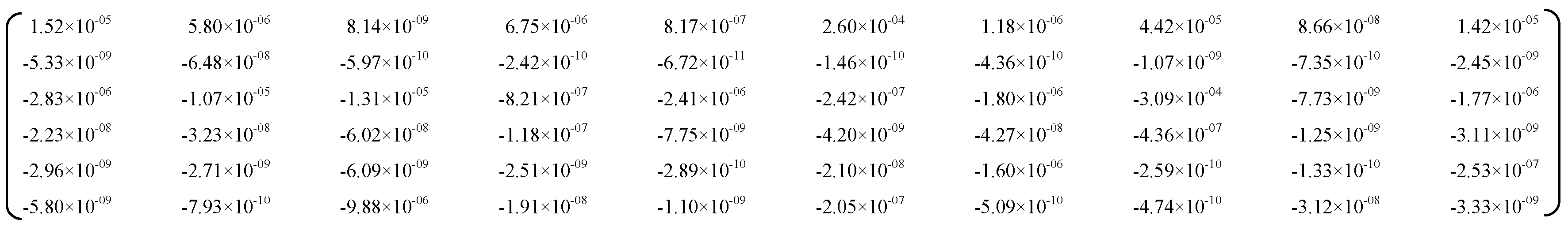
In this real-world situations, crisp values are insufficient. Many evaluation criteria are really imperfect and probably influenced by uncertain factors. Fuzzy method is used by many researchers in the literature, as considering human judgement of preferences is often unclear and hard to estimate by exact numerical values. We constructed the fuzzy neural network according to the dimensions of the training samples, and then determined the number of inputs/outputs of the fuzzy neural network and the fuzzy membership function number. Finally, we built membership function using Gauss the function fuzzy reasoning and sum-product. The function center value b and function witch value c are shown in Figure 4 and Figure 5, respectively. The ambiguity resolution used the weighted average method.

The normalized data was used for the training neural network, and we then used the trained fuzzy neural network to comprehensively evaluate the surface water quality. Results and rankings are shown in

Table 8. Alternatives and ranking according to Takagi-Sugeno Fuzzy Neural Network (TS-FNN).

Site	Global Performance	Ranking
$A_1$	−0.9959	1
$A_2$	−0.8015	2
$A_3$	−0.2747	4
$A_4$	0.0138	5
$A_5$	0.5008	6
$A_6$	−0.3872	3

.

4.7. AHP Evaluation

One of the advantages of AHP is the possibility to evaluate quantitative and qualitative criteria and alternatives on the same preference scale [54]. Similarly, we used AHP to evaluate all the indicators of surface water quality. In particular, a decision matrix $V={\left(v_{ij}\right)}_{n\times n}$ was first constructed, as shown in

Table 9. Surface water quality evaluation indicator matrix.

	${\mathit{F}}_1$	${\mathit{F}}_2$	${\mathit{F}}_3$	${\mathit{F}}_4$	${\mathit{F}}_5$	${\mathit{F}}_6$	${\mathit{F}}_7$	${\mathit{F}}_8$	${\mathit{F}}_9$	${\mathit{F}}_{10}$
$F_1$		1/2	3/2	1/3	5/3	7/6	2/3	1/6	4/3	5/6
$F_2$			8/3	2/3	3	2	4/3	1/3	7/3	5/3
$F_3$				2/7	8/7	5/7	3/7	1/7	6/7	4/7
$F_4$					7/2	5/2	3/2	1/2	3	2
$F_5$						2/3	1/3	1/6	5/6	1/2
$F_6$							1/2	1/4	5/4	3/4
$F_7$								1/2	2	3/2
$F_8$									3	2
$F_9$										1/2
$F_{10}$

, by the weights size from Table 3, which does not show a diagonal matrix. The final $CI=0.0126$, obtained through a consistency test, and $CR=0.0084<0.1$. Therefore, its mean value met the requirements.

Next, we constructed the matrix for each indicator. The indicator $Dissolved$ is shown as an example in

Table 10. $Dissolved$ indicator matrix.

	${\mathit{A}}_1$	${\mathit{A}}_2$	${\mathit{A}}_3$	${\mathit{A}}_4$	${\mathit{A}}_5$	${\mathit{A}}_6$
$A_1$		5/6	5/4	5/2	5	5/3
$A_2$			3/2	3	6	2
$A_3$				2	4	4/3
$A_4$					2	2/3
$A_5$						1/3
$A_6$

.

$CI=0$, as obtained through a consistency test, and $CR=0<0.1$, so its mean value also met requirements. Then, the eigenvalues of the criteria layer were found to be 0.2381, 0.2857, 0.1905, 0.0952, 0.0476, and 0.1429. Next, we computed the matrix of all evaluation indicators at criteria layer, as shown in

Table 11. Total evaluation indicator matrix at the criteria layer.

Site	${\mathit{F}}_1$	${\mathit{F}}_2$	${\mathit{F}}_3$	${\mathit{F}}_4$	${\mathit{F}}_5$	${\mathit{F}}_6$	${\mathit{F}}_7$	${\mathit{F}}_8$	${\mathit{F}}_9$	${\mathit{F}}_{10}$
$A_1$	0.2381	0.2857	0.2857	0.2381	0.2857	0.2500	0.2857	0.3000	0.2500	0.1818
$A_2$	0.2857	0.1905	0.2381	0.2857	0.2381	0.2500	0.2381	0.2000	0.1667	0.2727
$A_3$	0.1905	0.2381	0.1429	0.0952	0.1429	0.2500	0.1905	0.2000	0.1667	0.2727
$A_4$	0.0952	0.0952	0.0952	0.0476	0.0952	0.0833	0.0952	0.1500	0.1667	0.0909
$A_5$	0.0476	0.0476	0.0476	0.1429	0.0476	0.0417	0.0476	0.0500	0.0417	0.0455
$A_6$	0.1429	0.1429	0.1905	0.1905	0.1905	0.1250	0.1429	0.1000	0.2083	0.1364

.

As show in

Table 12. Alternatives and ranking according to Analytic Hierarchy Process (AHP).

Site	Global Performance	Ranking
$A_1$	0.2612	1
$A_2$	0.2355	2
$A_3$	0.1851	3
$A_4$	0.1024	5
$A_5$	0.0531	6
$A_6$	0.1627	4

, final values from high quality to low quality were ordered as follows: $A_1>A_2>A_3>A_6>A_4>A_5$.

Consistent with the abovementioned final ranking, we found the order of $A_1>A_2>A_3>A_6>A_4>A_5$ by weighted voting from Table 6, Table 7 and Table 8 and Table 12 according to the ensemble vote, as shown in

Table 13. Global performance ranking with ensemble learning.

Site	TOPSIS	GRA	TS-FNN	AHP	H Value	Ranking
$A_1$	1	1	1	1	1.000	1
$A_2$	2	2	2	2	0.881	2
$A_3$	3	3	4	3	0.557	3
$A_4$	5	5	5	5	0.201	5
$A_5$	6	6	6	6	0.000	6
$A_6$	4	4	3	4	0.495	4

.

4.8. Discussion

The comprehensive use of the ensemble multi-MCDM method was applied to the trend analysis of surface water quality to provide effective support for governmental implementation of management strategies for reservoir water resources. After detecting the similarity in surface water quality between different sampling sites, a representative sampling site is selected to optimize from each sampling group. For example, the surface water quality of the Ma’anshan Reach of the Yangtze River was found to be best from the results of Table 13, so it may be used as a life water source. The spatial pattern of water quality can also help local governments understand the pollution status of the managed areas and protect their respective aquatic ecosystems. The ensemble multi-MCDM method can avoid inconsistencies among different MCDM methods and help to determine and manage priorities by emphasizing the regional distinctions.

Weights showed that the values of indicators represent the importance of pollution sources. Line C of Table 3 presents the rankings of all the indicators. We can see from line C of Table 3 that $Manganate\left(F_3\right)$, $NitriteNitrogen\left(F_5\right)$ and $TotalArsenic\left(F_9\right)$ rank higher than other features, implying that they play a dominant role in water pollution. In particular, the weights of these three factors account for 40.73% of the total, while other seven factors account for the other 59.27%.

5. Conclusions and Future Work

Surface water quality has a major impact on the sustainable development of cities, especially in developing countries. How to efficaciously evaluate the impacts of surface water quality on social and economic development is an important issue for sustainable urban development. Studies have shown that integrating ensemble vote with MCDM is an effective means to improve traditional MCDM technique. This study has illustrates the usefulness of the proposed multi-MCDM approach in combination with ensemble vote as a tool for the evaluation of surface water quality. By comparing the results of four comprehensive evaluation methods, we found that different methods evaluating the same sample can results in different evaluation scores. However, we need same ranking results of various evaluation methods to employ a combined approach. Ensemble vote can solve this problem. According to the characteristics of the comprehensive evaluation index system of water quality and the purpose of the evaluation, this paper has used the TOPSIS, GRA, AHP, and TS Fuzzy Neural Network to evaluate the surface water quality of the study samples.

Although all results of this study illustrate the effectiveness of multi-MCDM methods in extracting characteristics from surface water quality datasets, there are some limitations to be noted. The disadvantage of this study is that the pollution sources are not identified to enable a fully understanding of the temporal and spatial variations of surface water quality. Further studies on surface water quality parameters, including TEMP, pH, and NH₄–N, should be carried out [55]. These parameters can be further monitored for more accuracy and controlled. In addition, to obtain the contribution of different pollutants in each area, it is necessary to quantitatively evaluate pollution sources.

The purpose of this work is to explore water pollution evaluation, with the additional aim of improving water quality in the future. According to the influence of surface water quality evaluation, we hope that the government can put forward the countermeasures forth the management of water pollution in the future. Furthermore, based on the found compatibility between the compliance assessments and the practical surface water quality evaluation, a compatible grading evaluation and management scheme has been developed for better private and public decision-making.

References

- Programme, W.W.A. The United Nations World Water Development Report: Water in a Changing World; UNESCO Publishing; Berghahn Books: New York, NY, USA, 2009. [Google Scholar]
- Oki, T.; Kanae, S. Global hydrological cycles and world water resources. Science 2006, 313, 1068–1072. [Google Scholar] [CrossRef] [PubMed]
- Duan, W.; He, B. Emergency Response System for Pollution Accidents in Chemical Industrial Parks, China. Int. J. Environ. Res. Public Health 2015, 12, 7868–7885. [Google Scholar] [CrossRef] [PubMed] [Green Version]
- Wang, Q.; Yang, Z. Industrial water pollution, water environment treatment, and health risks in China. Environ. Pollut. 2016, 218, 358–365. [Google Scholar] [CrossRef] [PubMed]
- Tu, J. Spatial Variations in the Relationships between Land Use and Water Quality across an Urbanization Gradient in the Watersheds of Northern Georgia, USA. Environ. Manag. 2013, 51, 1–17. [Google Scholar] [CrossRef] [PubMed]
- Gorgoglione, A.; Bombardelli, F.A.; Pitton, B.J.; Oki, L.R.; Haver, D.L.; Young, T.M. Uncertainty in the parameterization of sediment build-up and wash-off processes in the simulation of sediment transport in urban areas. Environ. Model. Softw. 2019, 111, 170–181. [Google Scholar] [CrossRef]
- Shi, H.; Shao, M. Soil and water loss from the Loess Plateau in China. J. Arid Environ. 2000, 45, 9–20. [Google Scholar] [CrossRef]
- Issaka, S.; Ashraf, M.A. Impact of soil erosion and degradation on water quality: A review. Geol. Ecol. Landsc. 2017, 1, 1–11. [Google Scholar] [CrossRef]
- Al-Isawi, R.H.; Almuktar, S.A.; Scholz, M. Monitoring and assessment of treated river, rain, gully pot and grey waters for irrigation of Capsicum annuum. Environ. Monit. Assess. 2016, 188, 287. [Google Scholar] [CrossRef] [PubMed]
- Alisawi, R.H.K.; Scholz, M.; Alfaraj, F.A.M. Assessment of diesel-contaminated domestic wastewater treated by constructed wetlands for irrigation of chillies grown in a greenhouse. Environ. Sci. Pollut. Res. 2016, 23, 25003–25023. [Google Scholar] [CrossRef] [Green Version]
- Le, C.; Zha, Y.; Li, Y.; Sun, D.; Lu, H.; Yin, B. Eutrophication of Lake Waters in China: Cost, Causes, and Control. Environ. Manag. 2010, 45, 662–668. [Google Scholar] [CrossRef]
- Nasiri, F.; Maqsood, I.; Huang, G.; Fuller, N. Water quality index: A fuzzy river-pollution decision support expert system. J. Water Resour. Plan. Manag. 2007, 133, 95–105. [Google Scholar] [CrossRef]
- Karamouz, M.; Zahraie, B.; Kerachian, R. Development of a Master Plan for Water Pollution Control Using MCDM Techniques: A Case Study. Water Int. 2003, 28, 478–490. [Google Scholar] [CrossRef]
- Lad, R.K.; Desai, N.G.; Christian, R.A.; Deshpande, A.W. Fuzzy modeling for environmental pollution potential ranking of industries. Environ. Prog. 2010, 27, 84–90. [Google Scholar] [CrossRef]
- Li, L.; Shi, Z.H.; Yin, W.; Zhu, D.; Ng, S.L.; Cai, C.F.; Lei, A.L. A fuzzy analytic hierarchy process (FAHP) approach to eco-environmental vulnerability assessment for the danjiangkou reservoir area, China. Ecol. Model. 2009, 220, 3439–3447. [Google Scholar] [CrossRef]
- Chung, E.S.; Lee, K.S. Prioritization of water management for sustainability using hydrologic simulation model and multicriteria decision making techniques. J. Environ. Manag. 2009, 90, 1502–1511. [Google Scholar] [CrossRef] [PubMed]
- Tebaldi, C.; Knutti, R. The Use of the Multi-Model Ensemble in Probabilistic Climate Projections. Philos. Trans. A Math. Phys. Eng. Sci. 2007, 365, 2053–2075. [Google Scholar] [CrossRef]
- Kubler, S.; Robert, J.; Derigent, W.; Voisin, A.; Le Traon, Y. A state-of the-art survey & testbed of fuzzy AHP (FAHP) applications. Expert Syst. Appl. 2016, 65, 398–422. [Google Scholar] [Green Version]
- Baykasoglu, A.; Kaplanoglu, V.; Durmusoglu, Z.D.; Sahin, C. Integrating fuzzy DEMATEL and fuzzy hierarchical TOPSIS methods for truck selection. Expert Syst. Appl. 2013, 40, 899–907. [Google Scholar] [CrossRef]
- Choudhary, D.; Shankar, R. An STEEP-fuzzy AHP-TOPSIS framework for evaluation and selection of thermal power plant location: A case study from India. Energy 2012, 42, 510–521. [Google Scholar] [CrossRef]
- Hosseini, S.; Al Khaled, A. A hybrid ensemble and AHP approach for resilient supplier selection. J. Intell. Manuf. 2016, 1–22. [Google Scholar] [CrossRef]
- Tang, L.; Yu, L.; Wang, S.; Li, J.; Wang, S. A novel hybrid ensemble learning paradigm for nuclear energy consumption forecasting. Appl. Energy 2012, 93, 432–443. [Google Scholar] [CrossRef]
- Liu, Y.; Zheng, Y.; Liang, Y.; Liu, S.; Rosenblum, D.S. Urban Water Quality Prediction based on Multi-task Multi-view Learning. In Proceedings of the International Joint Conference on Artificial Intelligence, New York, NY, USA, 9–15 July 2016; pp. 2576–2582. [Google Scholar]
- Wang, Q.; Dai, H.N.; Wang, H. A Smart MCDM Framework to Evaluate the Impact of Air Pollution on City Sustainability: A Case Study from China. Sustainability 2017, 9, 911. [Google Scholar] [CrossRef]
- Lin, C.T.; Chang, C.W.; Chen, C.B. The worst ill-conditioned silicon wafer slicing machine detected by using grey relational analysis. Int. J. Adv. Manuf. Technol. 2006, 31, 388–395. [Google Scholar] [CrossRef]
- Jaramilloa, P.; Mullerb, N.Z. Air pollution emissions and damages from energy production in the U.S.: 2002–2011. Energy Policy 2016, 90, 202–211. [Google Scholar] [CrossRef]
- Angelov, P.P.; Filev, D.P. An approach to online identification of Takagi-Sugeno fuzzy models. IEEE Trans. Syst. Man Cybern. Part B 2004, 34, 484–498. [Google Scholar] [CrossRef]
- Haykin, S. Neural Networks and Learning Machines; Pearson: London, UK, 2009. [Google Scholar]
- Lee, A.H.I.; Chen, W.; Chang, C. A fuzzy AHP and BSC approach for evaluating performance of IT department in the manufacturing industry in Taiwan. Expert Syst. Appl. 2008, 34, 96–107. [Google Scholar] [CrossRef]
- Altenburger, R.; Aitaissa, S.; Antczak, P.; Backhaus, T.; Barcelo, D.; Seiler, T.; Brion, F.; Busch, W.; Chipman, K.; De Alda, M.L.; et al. Future water quality monitoring—Adapting tools to deal with mixtures of pollutants in water resource management. Sci. Total Environ. 2015, 512, 540–551. [Google Scholar] [CrossRef]
- Boyd, J. Compensating for Wetland Losses under the Clean Water Act. Environment 2002, 44, 43–44. [Google Scholar] [CrossRef]
- Zou, Z.; Yun, Y.; Sun, J. Entropy method for determination of weight of evaluating indicators in fuzzy synthetic evaluation for water quality assessment. J. Environ. Sci. 2006, 18, 1020–1023. [Google Scholar] [CrossRef]
- Liou, S.; Lo, S.; Wang, S. A Generalized Water Quality Index for Taiwan. Environ. Monit. Assess. 2004, 96, 35–52. [Google Scholar] [CrossRef]
- Icaga, Y. Fuzzy evaluation of water quality classification. Ecol. Indic. 2007, 7, 710–718. [Google Scholar] [CrossRef]
- Liu, L.; Zhou, J.; An, X.; Zhang, Y.; Yang, L. Using fuzzy theory and information entropy for water quality assessment in Three Gorges region, China. Expert Syst. Appl. 2010, 37, 2517–2521. [Google Scholar] [CrossRef]
- Shi, B.; Wang, P.; Jiang, J.; Liu, R. Applying high-frequency surrogate measurements and a wavelet-ANN model to provide early warnings of rapid surface water quality anomalies. Sci. Total Environ. 2018, 610–611, 1390–1399. [Google Scholar] [CrossRef] [PubMed]
- Büyüközkan, G.; Çifçi, G. A novel hybrid MCDM approach based on fuzzy DEMATEL, fuzzy ANP and fuzzy TOPSIS to evaluate green suppliers. Expert Syst. Appl. 2012, 39, 3000–3011. [Google Scholar] [CrossRef]
- Hanine, M.; Boutkhoum, O.; Tikniouine, A.; Agouti, T. Comparison of fuzzy AHP and fuzzy TODIM methods for landfill location selection. SpringerPlus 2016, 5, 501. [Google Scholar] [CrossRef] [PubMed]
- Chen, J.K.; Chen, I.S. Using a novel conjunctive MCDM approach based on DEMATEL, fuzzy ANP, and TOPSIS as an innovation support system for Taiwanese higher education. Expert Syst. Appl. 2010, 37, 1981–1990. [Google Scholar] [CrossRef]
- Almanza, V.; Batyrshin, I.; Sosa, G. Multi-criteria selection of an Air Quality Model configuration based on quantitative and linguistic evaluations. Expert Syst. Appl. 2014, 41, 869–876. [Google Scholar] [CrossRef]
- Ferreira, L.; Borenstein, D. A fuzzy-Bayesian model for supplier selection. Expert Syst. Appl. 2012, 39, 7834–7844. [Google Scholar] [CrossRef]
- Kartal, H.; Oztekin, A.; Gunasekaran, A.; Cebi, F. An integrated decision analytic framework of machine learning with multi-criteria decision making for multi-attribute inventory classification. Comput. Ind. Eng. 2016, 101, 599–613. [Google Scholar] [CrossRef]
- Peng, Y.; Wang, G.; Kou, G.; Shi, Y. An empirical study of classification algorithm evaluation for financial risk prediction. Appl. Soft Comput. 2011, 11, 2906–2915. [Google Scholar] [CrossRef]
- Ali, R.; Lee, S.; Chung, T.C. Accurate multi-criteria decision making methodology for recommending machine learning algorithm. Expert Syst. Appl. 2017, 71, 257–278. [Google Scholar] [CrossRef]
- Gomes, H.M.; Barddal, J.P.; Enembreck, F.; Bifet, A. A Survey on Ensemble Learning for Data Stream Classification. ACM Comput. Surv. 2017, 50, 23. [Google Scholar] [CrossRef]
- Wang, Q.; Xia, L.Y.; Chai, H.; Zhou, Y. Semi-Supervised Learning with Ensemble Self-Training for Cancer Classification. In Proceedings of the 2018 IEEE SmartWorld, Ubiquitous Intelligence & Computing, Advanced & Trusted Computing, Scalable Computing & Communications, Cloud & Big Data Computing, Internet of People and Smart City Innovation (SmartWorld/SCALCOM/UIC/ATC/CBDCom/IOP/SCI), Guangzhou, China, 8–12 October 2018; pp. 796–803. [Google Scholar]
- Aliahmadipour, L.; Torra, V.; Eslami, E. On Hesitant Fuzzy Clustering and Clustering of Hesitant Fuzzy Data. In Fuzzy Sets, Rough Sets, Multisets and Clustering; Number 671; Springer: New York, NY, USA, 2017; pp. 157–168. [Google Scholar]
- Saaty, T.L. How to make a decision: The analytic hierarchy process. Eur. J. Oper. Res. 1990, 48, 9–26. [Google Scholar] [CrossRef]
- Chang, K.H. Generalized multi-attribute failure mode analysis. Neurocomputing 2016, 175, 90–100. [Google Scholar] [CrossRef]
- Mon, D.L.; Cheng, C.H.; Lin, J.C. Evaluating weapon system using fuzzy analytic hierarchy process based on entropy weight. Fuzzy Sets Syst. 1994, 62, 127–134. [Google Scholar] [CrossRef]
- Environmental Quality Standards for Suface Water; Ministry of Environmental Protection: Beijing, China, 2002.
- Garciacascales, M.S.; Lamata, M.T. On rank reversal and TOPSIS method. Math. Comput. Model. 2012, 56, 123–132. [Google Scholar] [CrossRef]
- Tseng, M. Using linguistic preferences and grey relational analysis to evaluate the environmental knowledge management capacity. Expert Syst. Appl. 2010, 37, 70–81. [Google Scholar] [CrossRef]
- Ishizaka, A.; Labib, A. Review of the main developments in the analytic hierarchy process. Expert Syst. Appl. 2011, 38, 14336–14345. [Google Scholar] [CrossRef]
- Wu, Z.; Zhang, D.; Cai, Y.; Wang, X.; Zhang, L.; Chen, Y. Water quality assessment based on the water quality index method in Lake Poyang: The largest freshwater lake in China. Sci. Rep. 2017, 7, 17999. [Google Scholar] [CrossRef] [Green Version]
Figure 1.
Our proposed hybrid ensemble multi-model framework.
Figure 2.
Neural network training procedure.
Figure 3.
Numbers 1–6 represent the Ma’anshan Reach of the Yangtze River, Quarry River, Yushan River, Cihu River, Yushan Lake and Suoxi River, respectively.
Figure 4.
Neural network training value b.
Figure 5.
Neural network training value c.