
In Data Science projects, sometimes we encounter the "Curse of Dimensionality", in which we have too many features compared to the number of observations. This can be problematic when fitting a model to the data. A commonly used process is to apply dimensionality reduction techniques, such as Principal Component Analysis (a.k.a. PCA). PCA transforms the data into a new dimensional space, where each dimension is orthogonal to each other. The principal components are sorted from the ones that explain the highest to lowest variance. The assumption is that the principal components with highest variance, will be the most useful for solving our machine learning problem, such as predicting if a datapoint belongs to one of two classes. In other words, we believe that the interclass variance is larger than the intraclass variance. For example, if we have two classes in a data set which we want to classify, the principal component with highest variance would be the best feature that would allow us to separate the data. This assumption, although logical, may not always be true as we will demonstrate in this post.
PCA is an unsupervised technique, meaning that the model does not take into account the label of each data point. PCA looks at the data set as a whole and determines the direction of highest variance. Then it determines the next direction of highest variance which is orthogonal to the previous ones, and so on.
In Figure 1(A) below we observe data which has two features X1 and X2. We have indicated with arrows the direction of highest and lowest variance with PC1 and PC2, respectively. In Figure 1(B) we have redrawn the data after performing the PCA transformation. Note that PC1 and PC2 now belong to the x and y-axis, respectively. In Figure 1(C) and 1(D) we present the data where we have reduced the dimension to only one component, indicating that we have performed a dimensionality reduction from two dimensions to one. In this example, PC1 accounts for 97.5% of the variance, compared to 2.5% from PC2. Typically, we would only select the principal components with highest variance to further do some modeling. In this case we would only use PC1.

Figure 1: (A) Original data set showing X1 and X2, (B) Data transformed to its principal components 1 and 2, (C) Figure presenting only the projection of principal component 1, and (D) Figure presenting only the projection of principal component 2.
In Figure 2 we observe the same data set previously presented in Figure 1. In this case, each data point has been labelled as belonging to the red or blue group. The labels are separable by their direction of highest variance (PC1). Note that when we apply the principal component transformation, the results are the same as what is observed in Figure 1 because the PC algorithm does not take into account the label of the data points. Figure 2(C) and (D) show that once we reduce the data to one dimension, PC1 is the best choice to apply a classification algorithm, while ignoring PC2. It can be observed that in Figure 2(C) we can separate the red from the blue by assigning the data points on the left side a red label and the right side a blue label. This technique is what is typically used when we apply dimensionality reduction, and it will work well for this case.
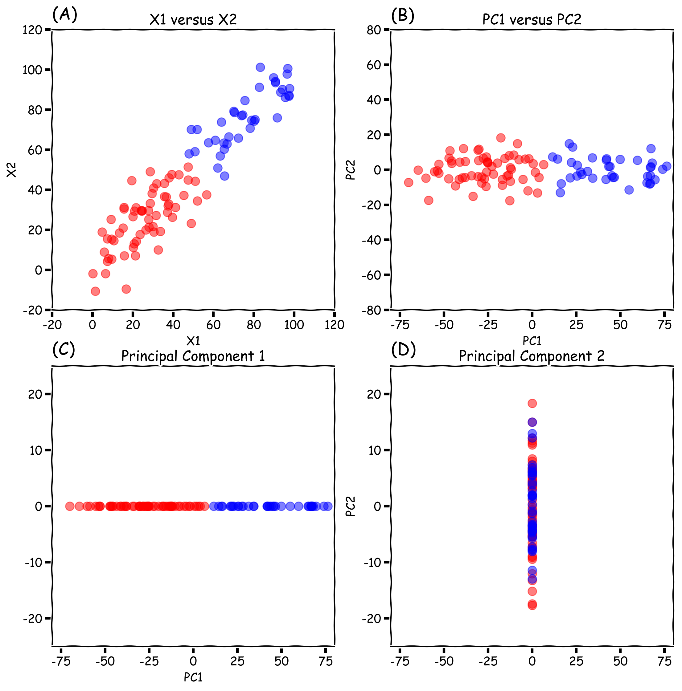
Figure 2: (A) Original data set showing X1 and X2, (B) Data transformed to its principal components 1 and 2, (C) Figure presenting only the projection of principal component 1, and (D) Figure presenting only the projection of principal component 2. In all cases the data is labeled with a strong separation on its direction of highest variance.
In Figure 3 we present the same data as before, but in this case we have labelled the data such that the separation of the classes is more pronounced in the direction of smaller variance. When we reduce the data to one dimension, we notice that the best separation occurs on PC2. Typically we would of have selected the direction of highest variance (PC1). As a result, we would have been using a feature that would not be effective to classify the data.

Figure 3: (A) Original data set showing X1 and X2, (B) Data transformed to its principal components 1 and 2, (C) Figure presenting only the projection of principal component 1, and (D) Figure presenting only the projection of principal component 2. In all cases the data is labeled with a strong separation on its direction of lowest variance.
In this post we have presented the ideas governing PCA for dimensionality reduction, in which we transform a data set into a new dimensional space without considering their labels (in an unsupervised manner). We then select the components that describe the majority of the variance, and use these as inputs to our machine learning challenge. The assumption is that the principal components with highest variance will also contain the most information that will allow us to separate data by its labels, as observed in Figure 2. However, when we view data sets where their separation is not on the highest variance, as observed in Figure 3, the use of the most important components of PCA will not work. This is a limitation for using PCA.
The code can be found here.