Clearing air around “Boosting”

By Puneet Grover, Helping Machines Learn.

Clearing Photo by SpaceX on Unsplash

Note: Although this post is a little bit math oriented, still you can understand core working of Boosting and Gradient Boosting by only reading first two sections i.e. Introduction and History. Sections after that are explanation of different Gradient Boosting algorithm’s papers.

This is one of the post from my posts from Concepts category, which can be found on my github repo here.

Index

1. Introduction
2. History (Bagging, Random Forest, Boosting and Gradient Boosting)
3. AdaBoost
4. XGBoost
5. LightGBM
6. CatBoost
7. Further Reading
8. References

NOTE:
This post goes along with Jupyter Notebook available in my Repo on Github:[ClearingAirAroundBoosting]

1) Introduction 

Boosting is an ensemble meta-algorithm primarily for reducing bias and variance in supervised learning.

Boosting algorithms, today, are one of the most used algorithms for getting state of the art results in a wide varieties of contexts/problems. And it has become a go to method for any machine learning problem or contest to get best results. Now,

1. What is the reason behind this massive success of Boosting Algorithms?
2. How it came to be?
3. What can we expect in the future?

I will try to answer all these questions, and many more, through this post.

2) History ^

Photo by Andrik Langfield on Unsplash

Boosting is based on the question posed by Kearns and Valiant (1988, 1989): “Can a set of weak learners create a single strong learner?”.

Robert Schapire’s affirmative answer in a 1990 paper to the question of Kearns and Valiant has had significant ramifications in machine learning and statistics, most notably leading to the development of boosting.

With Bagging there are a few other ensemble methods which came around the same time and you can say they are subset of modern Gradient Boosting algorithms, which are:

1. Bagging(Bootstrap Aggregating): (i.e. Bootstrapping + Aggregating)

Bagging is an ensemble meta-algorithm which helps in increasing stability and accuracy. It also helps in reducing variance and thus in reducing over-fitting.

In bagging, if we have N data points and we want to make ‘m’ models, then we will take some fraction of data [mostly, (1–1/e)≈63.2%] from data ‘m’ times and repeat some of the rows in them to make their length equal to N data points (though some of them are redundant). Now, we will train those ‘m’ models on these ‘m’ datasets and then get ‘m’ set of predictions. Then we aggregate those predictions to get final prediction.

It can be used with Neural Networks, Classification and Regression trees, and subset selection in Linear Regression.

2. Random Forest:

Random forests (or random decision forests) method is an ensemble learning method that operates by constructing a multitude of decision trees. It helps reduce overfitting which is common in Decision Tree models (with high depth value).

Random Forest combines “bagging” idea and random selection of features in order to construct a collection of Decision Trees to counter variance. As in bagging, we make bootstrapped training sets for decision trees, but now for each split that we make in tree generation process we only select a fraction of total number of features [mostly √n or log2(n)].

These methods, bootstrapping and subset selection, makes trees more uncorrelated with each other and helps reduce variance more, and thus reduces overfitting in more generalize-able manner.

3. Boosting:

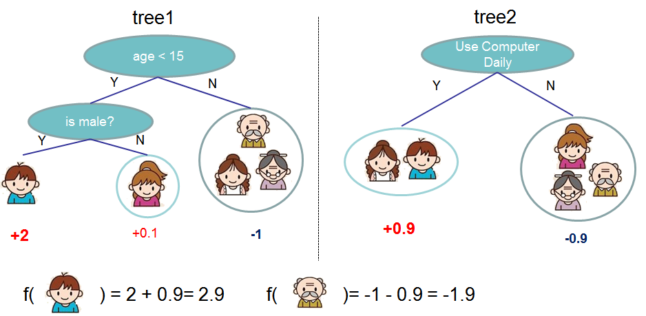
Above methods were using averaging of mutually exclusive models in order to reduce variance. Boosting is a little bit different. Boosting is a sequential ensemble method. For ‘n’ number of total trees, we add trees predictions in a sequential method (i.e. we add second tree to improve performance of first tree or you can say to tries to right the wrong of first tree, and so on). So what we do is, we subtract the prediction of first model multiplied by a constant (0<λ≤1) from the target values and then taking these values as target value we fit second model, and so on. We can see it as: new models trying to correct previous models/previous model’s mistakes. Boosting can be nearly summarized by one formula:

Example: Predicting if someone will like computer games. [Source: XGBoost docs]

I.e. final predictions are summation of predictions of all the models, each multiplied by a small constant (0<λ≤1). This is another way of looking at Boosting algorithm.

So, actually we try to learn small amount of information about target from each learner (which are all weak learners) which are trying to improve upon previous models and then sum them all to get final predictions (this is possible because we are fitting only to residuals from previous models). So, each sequential learner is trying to predict:

(initial predictions) — (λ * sum_of_all_predictions_of_previous_learners)

Each tree predictor can also have different λ value based on their performance.

4. Gradient Boosting: 

In gradient boosting, we take a loss function that is evaluated at every cycle of fitting (like in Deep Learning). First paper on Gradient Boosting by Jerome H. Friedman focused on additive expansion of the final function, similar to what we saw above.

We first predict a target value (say, γ), a constant which gives least error (i.e. first prediction is F0 = γ). After that we calculate gradients for every point in our dataset w.r.t. our previous output. So, we calculate gradient of error function w.r.t. sum of all outputs of previous models, which in case of Square Error will be:

gradient w.r.t. sum of all values for that data point (i.e. ith gradient)

By this we have gradients w.r.t. all outputs of previous models.

Why are we calculating gradients like this?

In Neural Networks it is straightforward to calculate gradients w.r.t. all the parameters (i.e. all neural nodes) because Neural Network is just linear (or some function whose gradient is easy to calculate) combination in all layers, so its easier to calculate gradients with Backpropagation (w.r.t. all parameters) and updating them. But here we can’t calculate gradient of output w.r.t. any parameters of a Decision Tree (like depth, number of leaves, split point …), because its not straightforward (actually its abstract).

1. H. Friedman used gradients of error (error function) w.r.t. every output and fitted model to those gradients.

How can this help in getting a better model?

What gradient w.r.t. each output represents is in which direction we should move and by how much to get to a better outcome for that particular data point/row, converting a Tree Fitting problem into Optimization Problem. We can use any kind of Loss Function, which is differentiable and which can be tailored specific to our task at hand, which was not possible with normal Boosting. For example, we can use MSE for regression tasks and Log Loss for classification tasks.

How are gradients used here to get better results?

Unlike in Boosting, where at ith iteration we learned some part of the output (target) and (i+1)th tree would try to predict what is left to be learned, i.e. we fitted to residuals, here in Gradient Boosting we calculate gradients w.r.t. all data points / rows, which tells us about the direction in which we want to move( negative gradients) and by how much (can be thought of as absolute value of gradient), and fit a tree on these gradients.

These gradients, based on our loss function (chosen to optimize our problem better than others), reflect change we would want for our predictions. For example in convex loss functions we will get some multiple to some multiple of exponential increase in gradients with increase in residuals, whereas residuals increase linearly. Therefore getting better convergence time. Depends on loss function and optimization method.

These gives us regions of gradients of data points which will need similar updates as they will have similar gradients. Now we will find best value for that region which will give least error for that region. (i.e. Tree Fitting)

After this we add these predictions to our previous predictions to get this stage’s final prediction.

Where γjm is prediction for jth region for mth tree and Jm is number of regions for mth tree. So adding γ, for that region found by tree fitting, times identity, giving 1 iff that data point is in current region..

Which gives us new predictions for every data point/row.

The basic difference between normal Boosting and GradientBoosting is that, in normal Boosting we fit our next model to residuals, whereas in GradientBoosting we fit our next model to gradients of residuals. Err… GradientBoosting actually uses a Loss Function, so we fit our next model to gradient of that loss function (where we find gradients by using previous predictions).

NOTE BEGIN

Further possible improvements to this:

Current Gradient Boosting libraries does much more than this, such as:

1. Tree Constraints (such as max_depth, or num_leavesetc)
2. Shrinkage (i.e. learning_rate)
3. Random Sampling (Row subsampling, Column subsampling) [At both tree and leaf level]
4. Penalized Learning (L1regression, L2 regression etc) [which would need a modified loss function and couldn’t have been possible with normal Boosting]
5. And much more…

These methods (some of them) are implemented in Boosting algorithm called Stochastic Gradient Boosting.

NOTE END

3) AdaBoost 

Photo by Mehrshad Rajabi on Unsplash

This is the first Boosting algorithm which made a huge mark in ML world. It was developed by Freund and Schapire (1997), and here is the paper.

In addition to sequentially adding model’s predictions (i.e. Boosting) it adds weights to each prediction. It was originally designed for classification problems, where they increased weights of all miss-classified examples and reduced weights of all data points classified correctly (though it can be applied to regression too). So, the next model will have to focus more on examples with more weight and less on examples with less weight.

They also have a constant to shrink every tree’s predictions, whose values is calculated during fitting and depend on error they get after fitting. More the error less is the value of constant for that tree. This makes predictions more accurate as we are learning less from less accurate models and learning more from more accurate learners.

It was originally for two class classification and chose outputs as {-1, +1}, where:

1. It starts with equal weight for every data point = 1/N (where, N: no. of data points),
2. Then it fits first classification model, h_0(x), to the training data using initial weights (which are same initially),
3. Then it calculates total error and based on that update weights for all data points (i.e. we increase weight of misclassified and decrease weight of those correctly classified). Total error also becomes useful in calculating shrinkage constantfor predictions of that particular tree. (i.e. we calculate constant, say α, which is small for large errors and vice versa, and is used both in shrinkage and weight calculation)

4. Finally current round’s predictions are added to previous predictions after multiplying with α. As it was originally to classify as +1 or -1, it takes sign of predictions after last round as final prediction:

where α_i is ith constant (prev. point) and h_i is ith model predictions

(AdaBoost is not Gradient based)

4) XGBoost

Photo by Viktor Theo on Unsplash

XGBoost tries to improve upon previous Gradient Boosting algorithms, to give better, faster and more generalizable results.

It uses some different and some new additions to Gradient Boosting, such as:

1. a) Regularized Learning Objective:

As in many other objective function’s implementations, here it proposes to add an extra function to the loss function to penalize complexity of the model(like in LASSO, Ridge, etc), known as the regularization term. This helps models not to overfit the data.

Some loss function + (Some regularization function to control complexity of model)

Now for Gradient Boosting, which is additive in nature, we can write our ‘t’ th prediction as F_t(x) = F_t-1(x) + y_hat_t(x), i.e. this rounds predictions plus sum of all previous predictions. Loss Function:

which after Taylor Series Approximation can be written as:

Where g_i and h_i are gradient and hessian of loss function. i.e. 1st order and 2nd order differentiation of loss function

Why till 2nd order?

Gradient Boosting with only first order gradient faces convergence issues (convergence only possible with small step sizes). And it is pretty good approximation of loss function, plus we don’t want to increase our computations.

Then it finds optimal value of loss function by putting gradient of loss function equal to zero and thus finding a function via Loss Function for making a split. (i.e. function for change in loss after split)

Found by putting above formla’s differentiation equal to zero. [Optimal Change value]

1. b) Shrinkage and Column subsampling:

It also adds shrinkage for every tree, to decrease influence of one particular tree, and subsampling of columns to combat overfitting and decrease variance as discussed in History section.

1. c) Different split finding algorithm:

Gradient Boosting algorithms goes through all possible splits to find the best split at that level. However, this can be a expensive bottleneck if our data is very large, so many algorithms use some kind of approximation or some other trick to find, not best but, a particularly good split. So, XGBoost looks at a particular feature’s distribution and selects some percentiles (or quantiles) as splitting points.

Note:
For approximate split finding these methods are also used, instead of percentile method:
1) By constructing approximate histogram of gradient statistics.2) By using other variants of binning strategies.

It proposes to selects a value, lets call it q, now from quantile range of [0, 100] nearly every qth quantile value is selected as candidate split point for splitting. There will be roughly 100/q candidate points.

It has also added Sparsity Aware split finding, which can be helpful in sparse BigData arrays.

1. d) For speed enhancement and space efficiency:

It proposes to divide data into blocks, in-memory blocks. Data in each block is stored in Compressed Column (CSC) format, in which each column is stored by corresponding feature value. So, a linear search of the column in block is sufficient to get all split points of that column, for that block.

Block format makes it easy to find all splits in linear time, but when it is turn to get gradient statistics for those points, it becomes a non-continuous fetches of gradient statistics (because gradients are still in previous format, where block-values have pointer to their gradient) which can lead to cache-misses. To overcome this problem, they made a Cache Aware algorithm for gradient accumulations. In it, every thread is given an internal buffer. This buffer is used to get gradients in mini-batch manner and accumulate them, in contrast to accessing some gradient from here and then some gradient from there in order.

Finding the best size of block is also a problem which can help use parallelism the best and reduces cache-misses the most.

It also proposes something called Block Sharding. It writes data on multiple disks alternatively (if you have those). So, when it wants to read some data, this setup can help read multiple blocks at the same time. For example if you have 4 disks, then those four disks can read 4 blocks in one unit time, giving 4x speedup.

5) LightGBM

Photo by Severin D. on Unsplash

This paper has proposed two techniques to speed up the overall Boosting process.

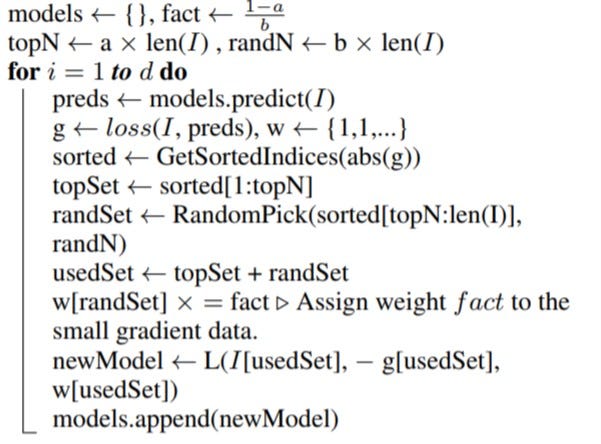
For first one, it proposes a method in which they won’t have to use all data points for a particular model, without loosing much information gain. It’s named Gradient Based One Side Sampling (GOSS). In it, they calculate gradients of the loss function and then sort them by their absolute value. It also has a proof to prove that values having larger value of gradient contribute more to information gain, so it proposes to ignore many data points with low gradient for that particular model.

So, take some fraction of top gradients and a different fraction from remaining (randomly from remaining gradients) for a particular model, with some low weight applied to random set of gradients as they have lower value of gradients and should not contribute much to our current model.

Get gradients of loss, sort them, take top gradient set and random from rest, reduce weight of random ones, and add this model to previous models’ set.

One thing to note here is that LightGBM uses histogram-based algorithms, which bucket continuous feature values into discrete bins. This speeds up training and reduces memory usage.

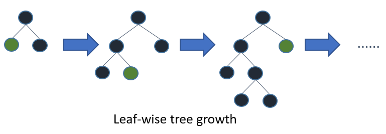
Also, they use a different kind of Decision Tree which optimizes leaf wise instead of depth wise that normal Decision Tree does. (i.e. it enumerates all possible leaves and selects the one with least error)

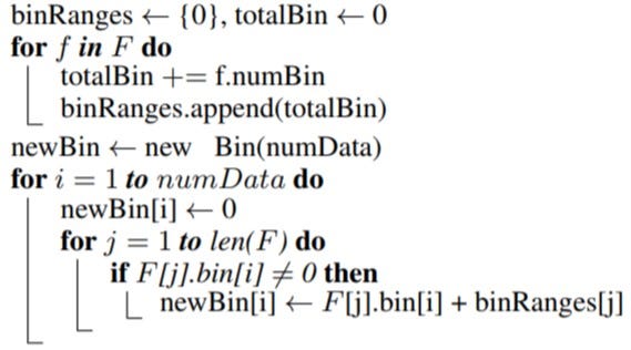
For the second one, it proposes a method in which to combine many features to make one new feature, thus reducing dimentionality of the data without much information loss. This method is called Exclusive Feature Bundling (EFB). It says that, in world of High Dimentional data there are a lot of columns that are mutually exclusive. How? As, high dimentional data has many columns which are highly sparse, there can be many columns present in data which are not taking any value at the same time (i.e. only one of them is taking a non-zero value most of the time, i.e. mutually exclusive). So, they have proposed to bundle such features into one, which don’t have conflict above some pre-specified value (i.e. they don’t have some non-zero value at same data point for many points. i.e. they are not fully mutually-exclusive, but mutually-exclusive till some level). Still to distinguish each value from different features, it proposes to add a different constant to values coming from different features, so values from one feature will be in one particular range and values from other features will not be in that range. For example, say we have 3 features to combine and all are between 0–100. So, we will add 100 to second feature and 200 to third feature to get three ranges for 3 features, equal to [0, 100), [100, 200) and [200, 300). And in tree based model this is acceptable, as it won’t affect information gain by splitting.

Find binRanges for all features to combine, make a new bin with values equal to bin_value + bin_range.

Making these bundles is actually NP-Hard problem and is similar to Graph Coloring problem which is also NP-Hard. So, as in Graph Coloring problem, it has opted for a good approximation algorithm instead of an optimal solution.

Although these two methods were the main highlight of this paper, it also provide those improvements to Gradient Boosting algorithms, like sub-sampling, max_depth, learning_rate, num_leaves etc., which we discussed above, in their package.

Overall this one is a quite mathematical paper. If you are interested in proofs, you should look into this paper.

6) CatBoost

Photo by Alex Iby on Unsplash

This paper focuses on one of the problem with Boosting suffers, i.e. leakage, target leakage. In Boosting, fitting of many models on training examples relies on target values (for calculating residuals). This leads to shift in target values in test set, i.e. prediction shift. So, it proposes a method to bypass this problem.

Plus, it also proposes a method for converting categorical features into target statistics (TS) (which can lead to target leakage if done wrong).

It has proposed an algorithm called Ordered Boosting which helps in preventing target leakage, and an algorithm for processing categorical features. Though both uses something called Ordering Principle.

Firstly, for converting categorical features into target statistics (TS). If you know about mean encoding or target encoding of categorical features, specially K-Fold mean encoding, it will be easy to understand as this is just a little twist to that. What they did to avoid target leakage, but still be able to do target encoding, is that for i-th element they took (i-1) elements above it, in dataset, to get feature value for this element (i.e. if 7 elements are above i-th element, of same category as the i-th element, then they took mean of target for those values to get feature value for i-th element).

Average target values if i,j belong to same category, only if in this iteration’s random permutation that element is above ith element (if condition in statement). ‘a’ and ‘p’ are parameters to save eq from underflowing.

Secondly, for making algorithm prediction shift proof, it has proposed an algorithm which they named Ordered Boosting. At every iteration, it samples a new dataset D_t independently and obtain unshifted residuals (as this is sufficiently/somewhat(depends) different dataset) by applying current model to this dataset and fit a new model. Practically, they add new data points to previous points, so, it gives unshifted residuals atleast for the new data points which are added in current iteration.

For i=1..n, from random permutation r`, compute avg(gradient if it belongs to same leaf) only if from permutation r` is that leaf point present above 2^(j+1) th point. [Update Model by adding new preds]

With this algorithm we can make ’n’ models if there are ’n’ examples. But we only make log_2(n) models, for time considerations. So, by this, first model is fitted to 2 examples, then second is fitted to 4 and so on.

CatBoost too uses a different kind of Decision Tree, called Oblivious Trees. In such trees the same splitting criterion is used across an entire level of the tree. Such trees are balanced and less prone to overfitting.

In oblivious trees each leaf index can be encoded as a binary vector with length equal to the depth of the tree. This fact is widely used in CatBoost model evaluator: it first binarizes all float features and all one-hot encoded features, and then uses these binary features to calculate model predictions. This helps in predicting at very fast speed.

7) Further Reading 

1. Trevor Hastie; Robert Tibshirani; Jerome Friedman (2009). The Elements of Statistical Learning: Data Mining, Inference, and Prediction(2nd ed.). New York: Springer. (ISBN 978–0–387–84858–7)
2. All References

8) References 

1. Wikipedia — Boosting
2. Trevor Hastie; Robert Tibshirani; Jerome Friedman (2009). The Elements of Statistical Learning: Data Mining, Inference, and Prediction(2nd ed.). New York: Springer. (ISBN 978–0–387–84858–7)
3. Paper — A Short Introduction to Boosting — Yoav Freund, Robert E. Schapire(1999) — AdaBoost
4. Paper — XGBoost: A Scalable Tree Boosting System — Tianqi Chen, Carlos Guestrin (2016)
5. Stack Exchange — Need help understanding XGBoost’s appropriate split points proposal
6. Paper — LightGBM: A Highly Efficient Gradient Boosting Decision Tree — Ke, Meng et al.
7. Paper — CatBoost: unbiased boosting with categorical features — Prokhorenkova, Gusev et al. — v5 (2019)
8. Paper — CatBoost: gradient boosting with categorical features support — Dorogush, Ershov, Gulin
9. Paper — Enhancing LambdaMART Using Oblivious Trees — Modr´y, Ferov (2016)
10. YouTube — CatBoost — the new generation of gradient boosting — Anna Veronika Dorogush
11. Gentle Intro to Gradient Boosting Algos — MachineLearningMastery

Original. Reposted with permission.

Resources:

• On-line and web-based: Analytics, Data Mining, Data Science, Machine Learning education
• Software for Analytics, Data Science, Data Mining, and Machine Learning

Related:

• Ensemble Learning: 5 Main Approaches
• Mastering The New Generation of Gradient Boosting
• The 10 Algorithms Machine Learning Engineers Need to Know