
Using Convolutional Neural Networks To Improve Road Safety And Save Lives
February 23, 2021

Applying AI on satellite images for improving road safety. We used pre-trained CNNs, VGG, ResNet, and Inception models to count vehicles on roads and analyze traffic flow to help save many lives.
The Why
At night, as you open the news, road crashes show up as if it has a scheduled time slot. As you go out in the morning, you find yourself being added to that sea of vehicles, you wonder,
“Can our roads be made safer or should we just suck it up?”
In the recent report released by United Nations titled — ” Sustainable Development Goals for 2020”, it was written:
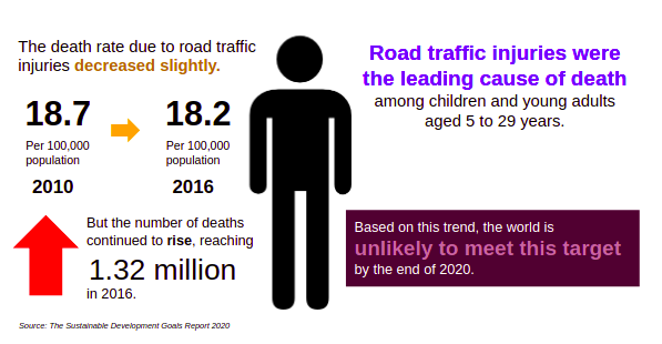
Infographic from Omdena
The United Nations recognizes this concern of road safety and listed it under Sustainable Development Goals 3 and 11 as seen below.
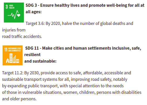
Photo from paho.org
This is not just a concern to be recognized by the United Nations,
“We all share the same roads; thus, the problem with road safety concerns us all.”
Contributing to the solution in increasing road safety, more than 30 machine learning engineers, subject matter experts, and mentors collaborated as part of an Omdena challenge to work towards iRAP’s vision of “a world free of high-risk roads.”
iRAP is a registered charity established to help tackle the devastating and economic cost of road crashes.
The challenge revolves around the three main objectives listed below. These are under the Ai-RAP initiative that aims to accelerate road assessments with the help of big data and AI.
Three main objectives of the challenge:
- Source geo-located crash data and produce iRAP Risk Maps of the historical crashes per kilometer and crashes per kilometer traveled for each road user
- Source road attribute, traffic flow, and speed data to the iRAP global standard and map the safety performance and Star Rating of more than 100 million km of road worldwide
- Produce repeatable road infrastructure key performance indicators that can form the basis of annual performance tracking
In this pipeline, we aim to contribute to the second objective by automatically sourcing the crucial component of vehicle count under the traffic or vehicle flow attribute using satellite imageries with the help of Artificial Intelligence.
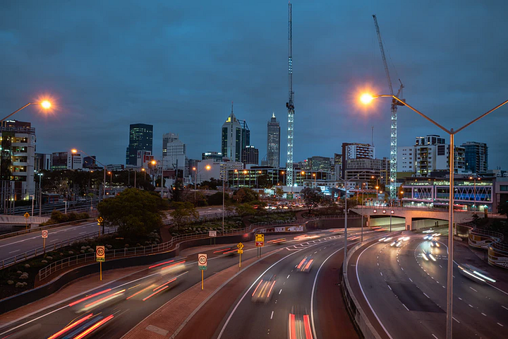
Flowing Vehicles Photo from Unsplash
According to iRAP, the vehicle flow attribute ranks as one of their priority attributes. Vehicles dominate the road as well as the reason for accidents. Thus, vehicle flow is one of the factors that influence the assessments regarding the road rating, and the estimations of the number of fatalities per 100m road segment. The higher the traffic flow, the higher a road user’s exposure to a certain crash such as a head-on collision.
Moreover, by automating the process, we can make this critical data more accessible and readily available to road authorities which have traditionally relied on other techniques, such as traffic counts at specific locations.
Overview of the Solution
Why choose satellite images?
We chose satellite images over ground-level data given its availability and advantage when it comes to occlusions. This is due to the nature that vehicles viewed in the ground level perspective offer the challenge of having multiple views of the vehicle such as partial occlusions due to other vehicles and other infrastructures. Even though vehicles viewed using satellite images lessen the possibility of such occlusions, another set of challenges are present in using satellite images.
A Regression Model instead of Object Detection
The objects in the satellite images are very small to detect and classify. Trying the state of the art deep learning algorithms such as YOLO did not give the required performance. Therefore, instead of detecting and counting, we focused on automatically giving the count of the vehicles given a whole satellite image tile that has approximately 100m road. In other words, counting the vehicles using satellite images is viewed as a regression problem instead of an object detection problem.
This approach is inspired by the paper — “Traffic density estimation method from small satellite imagery: Towards frequent remote sensing of car traffic.”
The Big Picture
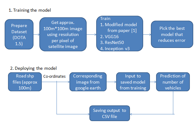
Source: Omdena
We divide our solution into two parts: the training phase and the deployment or the test phase. The training phase has the objective of picking the model with the lowest Root-Mean-Squared Error (RMSE) among four selected architectures given the training dataset. The deployment phase, on the other hand, acts as an automated system where the user input will be the shapefiles of the roads. We then collect the corresponding satellite imageries from those shapefiles and use the chosen best model from phase 1 to output the number of vehicles present in those roads.
Datasets and Data Preprocessing
There are two datasets used overall of which one is used for training and the other used for the testing in the deployment phase.
The DOTA v1.5 dataset
The dataset used in the training phase is from the DOTA v1.5 which contains 0.4 million annotated object instances within 16 categories and was originally sourced from Google Earth. The classes included are: plane, ship, storage tank, baseball diamond, tennis court, basketball court, ground track field, harbor, bridge, small vehicle, large vehicle, helicopter, roundabout, soccer ball field, swimming pool, and container crane.
Preprocessing the DOTA dataset
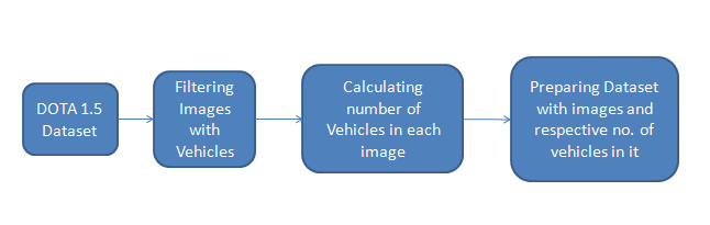
Preparing the DOTA v1.5 dataset. Source: Omdena
The process is shown in the figure above.
For each image, ground sample distance (gsd), with units in meters, refers to the physical size of one image pixel is given. Using this gsd, each image was preprocessed such that it was cropped for approx. 100-meter road. Further, we preprocessed the labels so that for each image tile, there will be a .txt file that contains the count of the vehicles. Lastly, we split it only to train and test sets and then have both datasets normalized by subtracting the mean and by dividing using the standard deviation.
Generating the Test Set
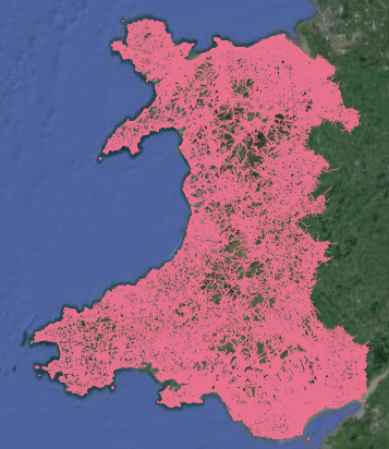
Whole Wales Shapefiles Dataset from OpenStreetMap
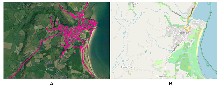
Sample Area. (A) Road Shapefiles overlayed on top of Google Earth imagery (B) Corresponding OpenStreetMap Imagery for reference
For the deployment phase, the input is a dataset full of road shapefiles. In this instance, we used the Wales shapefiles dataset from OpenStreetMap. From there, we chose a sample area in Abersoch to show the example predictions. These road shapefiles were preprocessed by slicing them to approx 100m road. The idea was that the users can use the shapefile to get any corresponding georeferenced image and then pass those images for prediction as seen below.
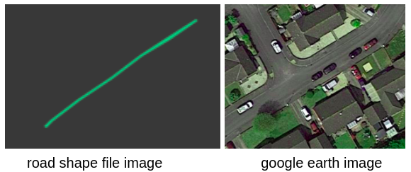
Generating the test set. Source: Omdena
For this pipeline, we collected the corresponding images from Google Earth. The images were further normalized by subtracting the mean and by dividing using the standard deviation before feeding to the models for prediction. A text file, road_coords.txt, was also created and contains information about the image name, and x and y coordinates with EPSG: 3857.
Models and Training
Four architectures with varying layer types were used, namely, a modified convolutional neural network from the paper before, VGG16, ResNet50, and Inceptionv3. These are commonly used as classification models but the trick on using them for regression lies in the output layer where we do not use any activation function and with only one unit for the Dense Layer.
In the following architectures, the other hyperparameters as listed below were held the same.
- input image: 300, 300, 3
- loss: mean-squared error (mse)
- optimizer: adam
- metrics: rmse
- epochs: 100
Modified Convolutional Neural Network
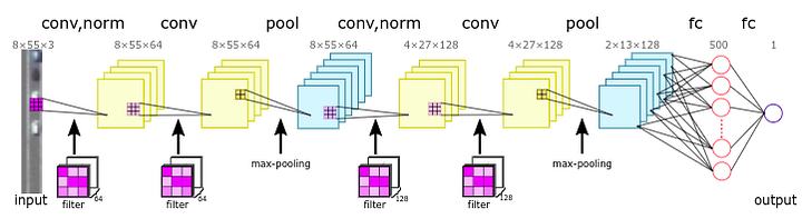
Original Network Structure from Traffic density estimation method from small satellite imagery: Towards frequent remote sensing of car traffic
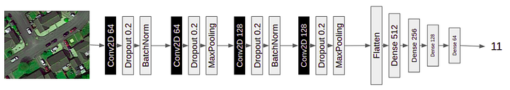
Modified Network Structure. Source: Omdena
As shown above, the original network structure was modified to add convolutional and dense layers, and Dropout for regularization. This model was trained from scratch and without transfer learning. Given that, it still achieved an RMSE of 4.5858.
VGG16
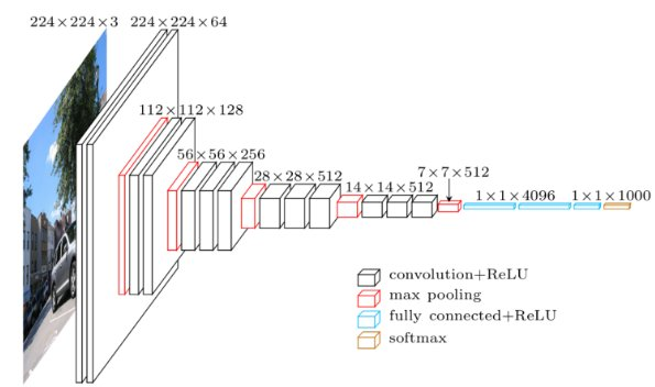
VGG16 from Image Source
The second model was VGG16 as seen above. Briefly, VGG16 is a sequential model with 16 layers composed of convolutional and dense layers. We used ImageNet as the pretrained weight. The layers were cut off in the block5_pool layer and Dense Layers were added. This model yielded the highest performance in the test set with an RMSE of 2.7688.
Residual Networks (ResNet)

ResNet50 from Image Source
ResNet50 is known for its residual block unlike the sequential nature of VGG16. ImageNet was also used as pretrained weights. We cut off a layer was max_pool and Dense layers were also further added. This model yielded an RMSE of 3.0782 which is second to VGG16.
Inception Network
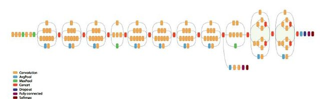
Inception V3 from Image Source
“To go deeper” is what Inception Networks are for. They introduced new concepts and layer types such as branching and concatenation layers. Like the others, ImageNet served as its pretrained weights. It was cut off at mixed7 layer and Dense Layers were also added after it. Among the models above, this model incurred the lowest performance with an RMSE of 6.1485.
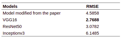
Summary of the RMSE results. Source: Omdena
Model Deployment
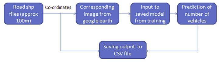
Model Deployment Pipeline. Source: Omdena
After selecting the model with the best RMSE, the generated test dataset was fed. The output was a CSV file containing the following information: image names, x and y coordinates (EPSG:3857), wkt_geom, and vehicle count predictions. This CSV file can be further visualized using QGIS and further can be used in the analysis along with other measures for rating the roads. The visualization of the sample area and a snapshot of its corresponding CSV file can be seen below.
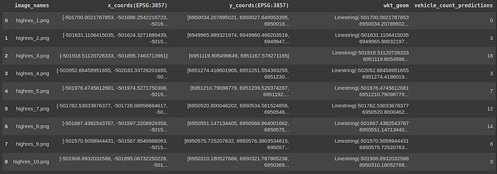
Snapshot of CSV file output viewed as dataframe. Source: Omdena
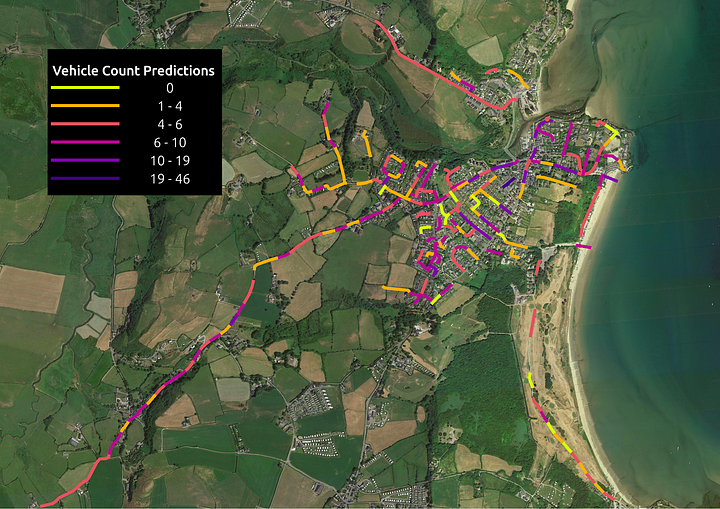
Visualization of the vehicle count predictions in the sample area. Source: Omdena
Conclusion and application
Technical improvements
Improvements could be done in order to make the model more robust such as extracting the road first and consider objects only on the road, if there are no shapefiles available for a place, adding road segmentation in the pipeline, and turning the predictions to shapefiles that may serve as an alternative, etc. We could also play around with data, model architectures, and hyperparameters to achieve better performance.
How the solution will be applied
In this pipeline, we built a model to automatically source the crucial component of vehicle count under the traffic or vehicle flow attribute using satellite imageries and neural networks. This information can be further integrated into the road safety analysis of iRAP´s global standard and help to map the safety performance and Star Rating of more than 100 million km of road worldwide.
—
This article is written by Lois Anne Leal and Chaitree Sham Baradkar.
Ready to test your skills?
If you’re interested in collaborating, apply to join an Omdena project at: https://www.omdena.com/projects
Related Articles


