LiDAR-Based Estimates of Canopy Base Height for a Dense Uneven-Aged Structured Forest
by
 , , and
Alexandra Stefanidou
1,*, 
Ioannis Z. Gitas
1 ,
,
Lauri Korhonen
2,
Dimitris Stavrakoudis
1 and
and
Nikos Georgopoulos
1 
1
Laboratory of Forest Management and Remote Sensing, Department of Forestry and Natural Environment, Faculty of Agriculture, Forestry and Natural Environment, Aristotle University of Thessaloniki, P.O. Box 248, 54124 Thessaloniki, Greece
2
University of Eastern Finland, School of Forest Sciences, P.O. Box 111, FI-80101 Joensuu, Finland
*
Author to whom correspondence should be addressed.
Remote Sens. 2020, 12(10), 1565; https://doi.org/10.3390/rs12101565
Submission received: 2 April 2020
/
Revised: 26 April 2020
/
Accepted: 10 May 2020
/
Published: 14 May 2020
(This article belongs to the Section Forest Remote Sensing)
Abstract
:Accurate canopy base height (CBH) information is essential for forest and fire managers since it constitutes a key indicator of seedling growth, wood quality and forest health as well as a necessary input in fire behavior prediction systems such as FARSITE, FlamMap and BEHAVE. The present study focused on the potential of airborne LiDAR data analysis to estimate plot-level CBH in a dense uneven-aged structured forest on complex terrain. A comparative study of two widely employed methods was performed, namely the voxel-based approach and regression analysis, which revealed a clear outperformance of the latter. More specifically, the voxel-based CBH estimates were found to lack correlation with the reference data (, ) while most CBH values were overestimated resulting in an of . On the contrary, cross-validation of the developed regression model showcased an , and of , and respectively. Overall analysis of the results proved the voxel-based approach incapable of accurately estimating plot-level CBH due to vegetation and topographic heterogeneity of the forest environment, which however didn’t affect the regression analysis performance.
1. Introduction
Canopy base height (CBH)—although not universally defined—commonly refers to the vertical distance between ground surface and the base of the continuous live crown (i.e., lowest branch of the tree crown with live foliage) [1,2,3,4,5]. Either on stand or individual tree level, CBH constitutes one of the most important forest structure parameters in several forestry applications. It can be used as an indicator of tree foliage amount and seedling growth [6,7,8], for wood quality estimation [9,10], for crown conditions and forest health evaluation [6,11] as well as in fire behavior prediction systems such as FARSITE, FlamMap and BEHAVE [12,13,14,15,16].
Despite being essential for forest and fire managers, the challenge of CBH information acquisition still remains unresolved. Field surveys, while the most reliable and accurate method for obtaining CBH information, are particularly labor-intensive, costly, time-consuming and sometimes even restricted when the study area is inaccessible [17,18]. Remote Sensing technology has provided an alternative solution for monitoring forest parameters with higher time and cost-efficiency. In particular, Light Detection and Ranging (LiDAR) sensors can penetrate forest canopies and has been proven to successfully retrieve vertical structure information including measures of individual and plot level CBH [18,19,20,21,22,23].
Since LiDAR is a rather contemporary technology and under continuous development, LiDAR-based CBH prediction still constitutes an emerging and current topic. Most LiDAR-derived CBH estimation methods found in the literature so far are based either on regression analysis or direct estimations [1]. Regression-based methods establish empirical relationships between field measurements and LiDAR-derived features in order to create predictive models which can be applied on other areas with similar vegetation and topography conditions [24]. For instance, Botequim et al., (2019) developed a regression model for plot-level CBH prediction in pine and oak stands of Southwestern Spain. The model presented an adjusted coefficient of determination (adj.) between 0.75–0.98, which was similar or higher compared to other studies [25]. Kelly et al., (2017) predicted plot-level CBH for a mixed pine forest over complex terrain in California (USA) using regression analysis which resulted in a predictive model of and m [26]. LiDAR-derived variables were also used for CBH estimation in pure and even-aged pine stands in Asturias (NW Spain) [27]. The fitted model presented an of while the cross-validation revealed an (i.e., adjusted model efficiency measure) equal to [27]. In 2014, Hermosilla et al., introduced a method which employs full-waveform LiDAR-derived metrics and regression analysis to retrieve CBH information for a forested watershed primarily dominated by Douglas-fir in US Oregon. The predictive model was cross-validated presenting an , , and of , m, and respectively [4]. Erdody and Moskal (2010) compared the individual and combined use of LiDAR data and near-infrared imagery for estimating canopy parameters of individual trees including CBH. The results showcased that LiDAR alone significantly outperformed the near-infrared imagery ( vs. ) while the combined use of these data slightly improved the fit of the regression model () [20].
Contrary to regression-based CBH prediction, direct methods are based exclusively on the vertical profile analysis of LiDAR points and can be applied without prior knowledge about the vegetation conditions of the study area. The most recent example is the method introduced by Luo et al., (2018) for direct CBH retrieval of individual trees in the steep terrain of Tahoe National Forest in California (USA). The comparison between the field measured and predicted CBH revealed an and of and m respectively [1]. A voxel-based approach was also employed by Popescu and Zhao (2018) [3] who analyzed the LiDAR vertical structure of delineated individual conifer and deciduous trees for CBH estimation. The results showed that conifer CBH was more accurately estimated () compared to deciduous trees (). In 2010, Vauhkonen et al., examined the potential of Delaunay triangulations and alpha shapes in estimating CBH for pine trees in eastern Finland and compared this method with alternative approaches from earlier studies. Although alpha-weighted Delaunay triangulation method performed well ( = 3–3.5 m), the results underperformed the reference methods which estimated CBH with of approximately 2 m [28]. Dean et al., (2009) directly estimated CBH from LiDAR data in a mature, even-aged pine stand in H.G. Lee Memorial Forest of Louisiana USA. The method was based on point cloud voxelization and data fitting to Weibull distribution resulting in a statistically significant overestimation, which however can be eliminated by linear equation with reference data [29].
Studies have also focused on the examination of the combined employment of LiDAR vertical profile and regression analysis for reliable CBH prediction. A prominent example is the research of Maguya et al., (2015) who analyzed the LiDAR vertical structure through voxelization in order to derive new LiDAR metrics and used them as independent variables in a linear regression for plot-level CBH estimation in Koli Forest (Eastern Finland) [22]. The results revealed that the use of new metrics instead of the traditional percentiles gave more accurate CBH estimates (i.e., , vs. , ).
Despite the promising reported results, the aforementioned CBH prediction approaches have both advantages and limitations. On one hand, direct estimation methods don’t rely on field measurements facilitating their application even to inaccessible areas without reference data [30]. On the other hand, reliable analysis of LiDAR vertical profiles requires adequate pulse penetration capabilities (i.e., presence of points from the lower part of the canopy) which strongly depend on the sensor characteristics and several vegetation, topography and weather conditions such as canopy cover, presence of steep slopes and relative air moisture [18,31]. Predictive models constructed by regression analysis are not as sensitive to pulse penetration as the former approach but essentially rely on field data. In fact, the quantity and quality of sample plots may significantly affect the estimation accuracy. Furthermore, such models tend to be species and site specific which means that their applicability to different areas may be limited [16].
To the best of our knowledge, very few researches have focused on the comparative study of these two approaches in a specific study area. Sumnall et al., (2016) and Maltamo et al., (2018) performed regression and vertical profile analysis for CBH estimation at the plot and individual tree level in pine-dominated forests of USA and Finland respectively [18,32]. Both studies concluded that regression models performed better compared to the vertical distribution analysis.
The aim of the present study was to examine the potential of airborne LiDAR data to accurately estimate CBH at the plot-level in a dense hybrid fir (Abies borisii regis) forest characterized by uneven-aged structure on complex terrain. The study investigates and compares the afore-described widely used approaches through the implementation of high-density LiDAR point clouds and area-based metrics. The specific objectives were to:
- apply a voxel-based approach to estimate CBH directly from LiDAR data at the plot-level,
- perform a plot-level regression analysis to estimate CBH through the implementation of LiDAR-derived metrics and
- evaluate the accuracy of the CBH estimates and compare the applied methods.
Taking all the surrounding literature into account, we acknowledge that both methods can theoretically achieve high estimation accuracies in our study area and that the regression-based method is supposed to outperform the voxel-based approach. Nevertheless, previous studies have also suggested the exclusive use of the voxel-based approach for CBH estimation [1,3,28,29]. In addition, the reported studies focus mainly on pine species over different topographic conditions which can reflect on the acquired LiDAR point cloud structure and eventually facilitate or hinder accurate CBH predictions. Considering that each method has advantages and limitations, it is of utmost importance to quantify the level of their accuracy and the difference between the results, if any, even if they prove to be consistent with the already reported ones. For instance, the regression model may have had a better performance but the RMSE derived from the voxel-based method could be still sufficiently low for practical applications. Under these circumstances, a cost benefit analysis could lead to the application of the voxel-based approach in case the area under examination was inaccessible or economic constraints did not allow field measurements. It should be noted that such challenges are common in Greece since it constitutes one of the most mountainous countries in Europe.
Consequently, despite the highly accurate results reported in the literature, there is still a profound need to reach the aim of this study, the results of which can form the basis for future work and development of more sophisticated and accurate CBH prediction methods.
2. Study Area and Dataset Description
2.1. Study Area
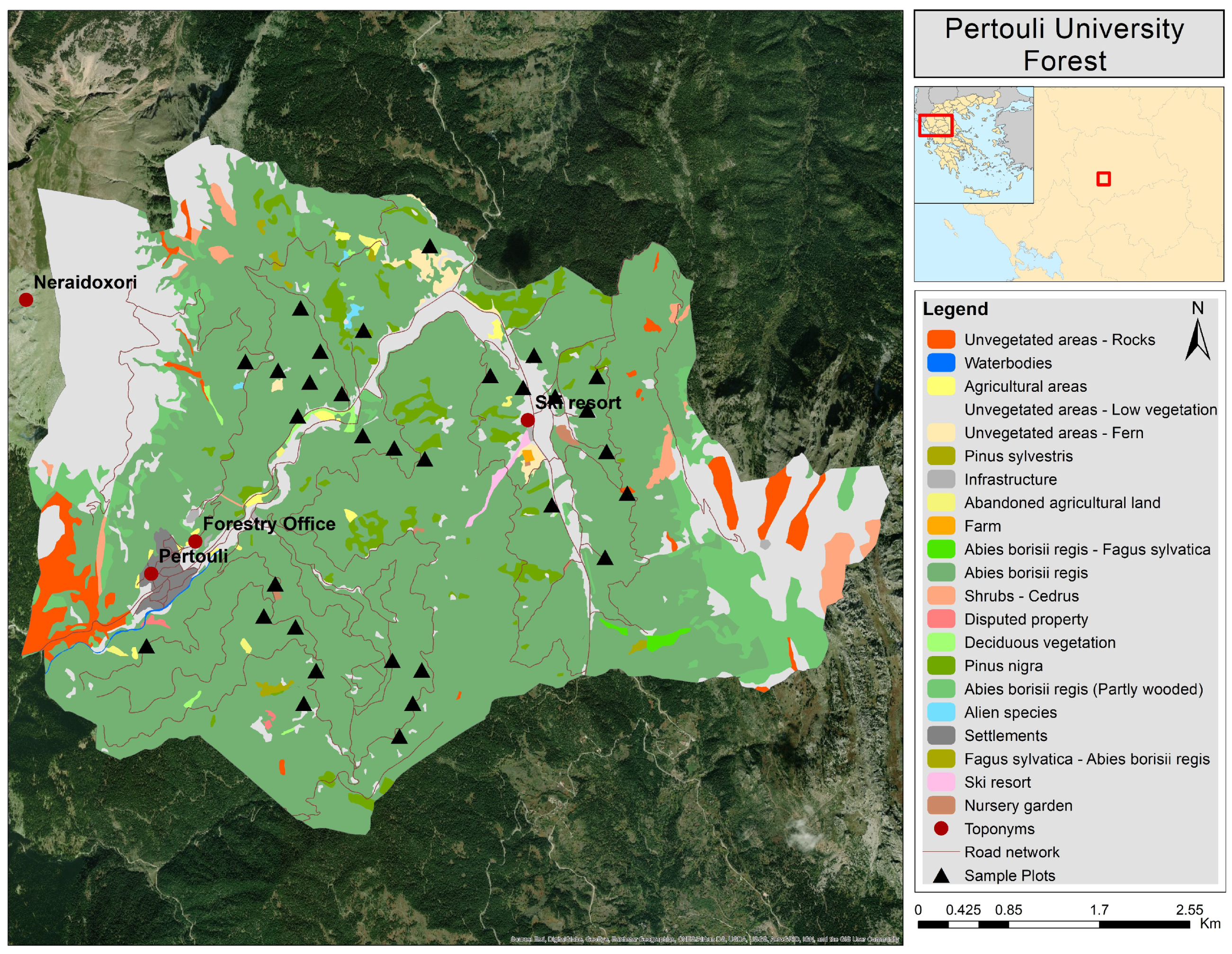
The present study was conducted at the Pertouli University Forest located in the Pindos Mountain Range of Central Greece (latitude 3932–3935 and longitude 2133–2138) (Figure 1). The forest extends from the western slopes of Koziakas Mt. (1901 m) to the northeastern slopes of Boudoura Mt. (2067 m) occupying an area of 3296.59 ha. 2427.62 ha of the area is forest or partly forested, 130.74 ha non-vegetated areas within the forest, 555.40 ha mountain pastures, 114 ha lowland grasslands and 68.83 ha are occupied by agricultural areas and settlements.
Elevation ranges from 1100 m to 2073 m above mean sea-level and the climate is characterized as transitional (i.e., Mediterranean-Mid-European) with rainy and cold winters and relatively warm and dry summers. The forest predominantly consists of natural hybrid Abies borisii regis (Abies alba Mill. X Abies cephalonica Loud.) pure stands. The understorey vegetation (i.e., natural regeneration) comprises mainly Abies borisii regis species as well. The forest presents an uneven-aged structure due to the shade-tolerance of this species, which enables the survival of young regeneration under the shade of adjacent trees for a prolonged period of time and penetration into the midstory once light and growing space conditions become favorable.
2.2. Dataset Description
2.2.1. Airborne LiDAR data
LiDAR data were acquired in October 2018 over the entire area of the Pertouli University Forest using a RIEGL VQ-1560i-DW laser scanner sensor mounted on an airplane (detailed sensor specifications can be found at http://www.riegl.com/nc/products/airborne-scanning/produktdetail/product/scanner/55/). An average flying altitude of 2243 m above the mountainous terrain and a maximum scan angle rank of off nadir were used. The scanner includes two laser channels of different wavelengths, namely the Green (532 nm) and Near Infrared (1064 nm).
2.2.2. Field Measurements
Field measurements were conducted during the fall of 2019. The one-year temporal gap between the LiDAR data acquisition and field work is considered negligible as the difference of plot-level CBH is insignificant. CBH was measured in 32 plots (Figure 1) of 1000 m each (rectangle m) covered by pure dense Abies borisii regis stands. The selection of the specific plot dimensions was based on the sampling method which is applied in the study area for the forest management plan development and constitutes one of the two methods (fixed-area plots of size m or Bitterlich plots) employed in the framework of all forest management plans in Greece. The distribution of plots was performed in a way to represent a variety of elevations, aspects, slopes and tree densities over the study area (Table 1), although the accessibility of the area and vegetation cover (partly wooded stands were avoided) was also taken into account. Plots subjected to any natural or human interventions during the time period between the LiDAR flight and field work were not included in the sample dataset.
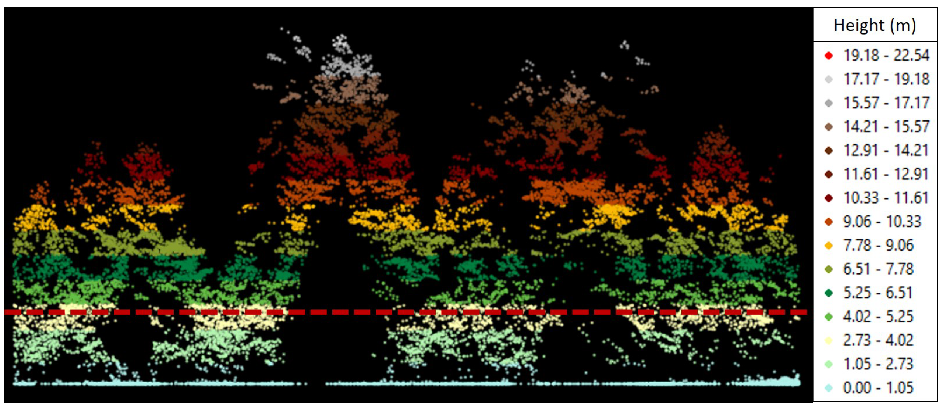
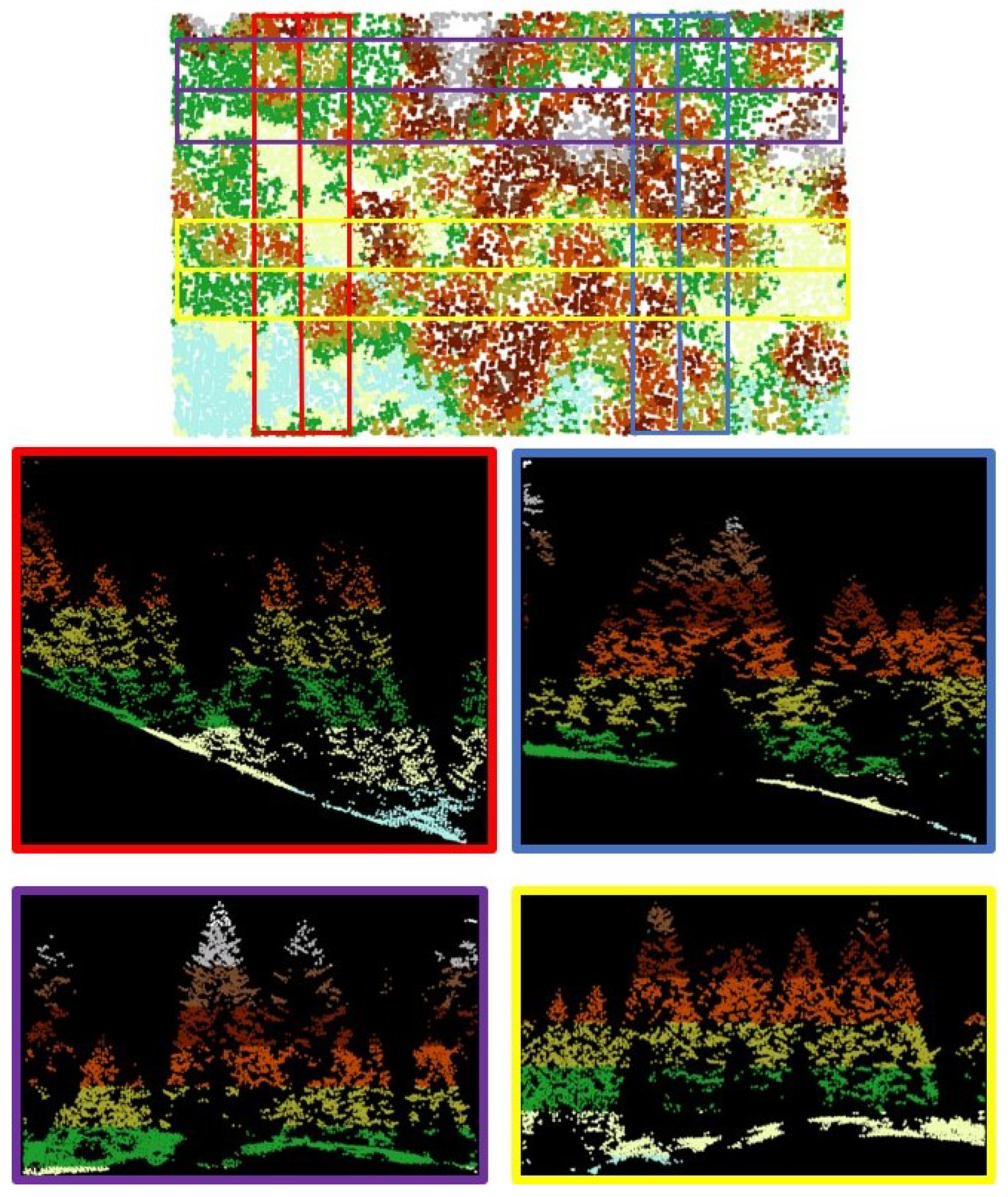
The plots’ location was recorded using a handheld GPS with an average horizontal accuracy of 3 m. Within each plot, the diameter at breast height (DBH) of all trees (i.e., 54 trees per plot on average) was recorded and the CBH of ten trees from all DBH classes (i.e., I: 4–20 cm, II: 21–34 cm and III/IV: 35–82 cm) was measured. The height of lowest branches with live foliage which were isolated from the main tree crown was not considered as crown base [2,3,5]. The plot-level CBH was subsequently calculated as the weighted average considering the proportion of trees of each DBH class in the plot. Figure 2 presents an illustration example of the field-measured average CBH of plot 29 (Table 1) on the respective height-normalized LiDAR point cloud.
It should be noted that prior to adopting the above-described sampling method, we measured all trees in eight of the plots and the plot-level CBH was computed as the arithmetic mean of all CBH values. The comparison of the plot-level CBH derived from both sampling methods revealed an average difference of 0.33 m which can be actually attributed to the precision (i.e., 0.5 m) of the instrument used for the measurements (i.e., Blume-Leiss altimeter) and/or measurement errors of random nature, such as leaning trees or branches obscureness due to dense canopy [33]. To this end, we concluded that the measurement of a sample of trees per plot is sufficient for the derivation of reliable reference data. Although we acknowledge the additional uncertainty that the specific sampling method may introduce in some plots, the measured data are as reliable as they could reasonably be.
3. Methods
3.1. Lidar Data Preprocessing
“Prior to delivery, the LiDAR data were preprocessed by the contractor, namely GEOSYSTEMS HELLAS S.A. (https://www.geosystems-hellas.gr/en/home/). The wavelengths were initially transformed to discrete returns (maximum of seven returns per transmitted pulse) resulting in point density of approximately 19 points m for each channel (Green and NIR). The point clouds were subsequently georeferenced, atmospherically corrected and the noise was reduced (e.g., multiple-time-around echoes elimination). The final point cloud was produced by merging the data of the two channels (without maintaining the information about the channel each point belongs to), removing any duplicated points and classifying the remaining ones into six classes, namely ground, low, medium, and high vegetation, buildings and low point noise.
The overlap between adjacent strips, which ensured a spatially continuous coverage of the surveyed area, along with the afore-described preprocessing resulted in an average point density of 82.99 points m with a scan angle rank from to 32 and a point spacing of 0.4 m.”
3.2. Voxel-Based CBH Estimation
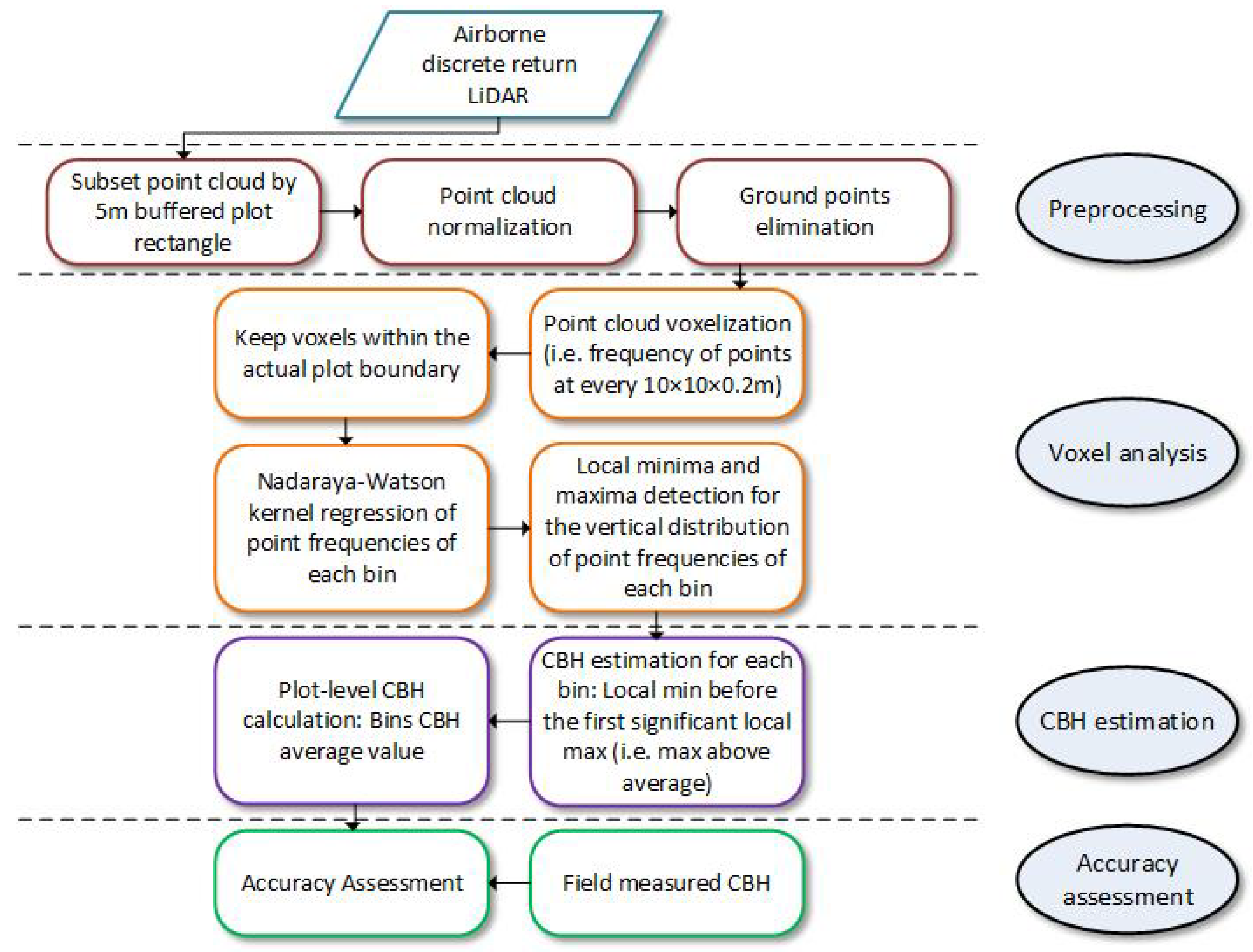
The voxel-based method applied in this study is based exclusively on the vertical point height distribution (Figure 3). The concept was to analyze the points frequency in the vertical profile and identify the height where it rises considerably over the average frequency value of the entire profile.
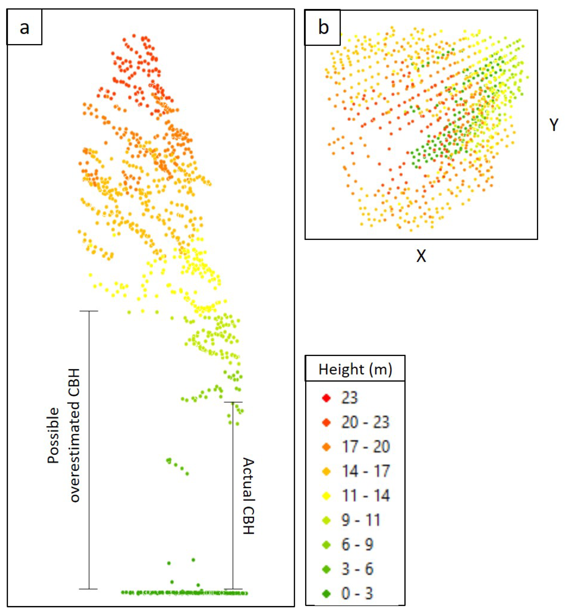
First, the rectangle vector file of each plot buffered by 5 m was used for the extraction of the respective point clouds. The 5 m area around the plot was used to avoid the vertical cut of tree canopies located on the plot edges which create considerable gaps and eventually cause CBH overestimation (also known as edge effect) (Figure 4). The point cloud of each plot was height-normalized using k-nearest neighbor approach with an inverse-distance weighting (kNN-IDW) and ground points were eliminated.
The removal of understorey vegetation points has been adopted in other voxel-based methods (e.g., [1,20]) in order to eliminate the impact of shrubs and small trees on CBH estimation accuracy. Nevertheless, considering the forest’s structural characteristics, this step was considered inappropriate for two reasons. First, as mentioned in Section 2.1, the forest is characterized by an uneven-aged structure leading to an overlap of the top of high understorey vegetation—where present—with the CBH. Additionally, a lack of points from very low vegetation was observed in the majority of the sample plots. Based on the above, additional analysis for the removal of understorey vegetation would either have no impact on the CBH prediction accuracy or cause overestimation since points from the actual CBH would be removed.
The preprocessing was followed by the voxelization of the point clouds at a resolution of m (). Each voxel (3D pixel) contained a single value of the number of included LiDAR returns. The selection of the optimal voxel size was influenced by the point cloud spacing and spatial distribution and was achieved through the examination of a variety of voxel sizes and their effect on the resulting CBH prediction accuracies [22]. It was observed that horizontal voxel dimensions lower than 10m resulted in a very low number of points in multiple voxels leading to the identification of false abrupt increases in the point frequencies of the vertical point cloud profile. Furthermore, the presence of considerable within canopy gaps (clearly visible in Figure 2 of the revised manuscript) led to the generation of a series of vertically adjacent zero-frequency voxels resulting in a considerable CBH overestimation. On the contrary, when a larger horizontal voxel size was applied, small gaps and significant increases in the vertical point frequency distribution were omitted. The vertical voxel size of 0.2 m was selected based on the desired precision of the estimated CBH values. In particular, a vertical size lower than 0.2 m created multiple voxels of zero frequency, similarly to the use of small horizontal voxel size, but heights greater than 0.2 m resulted in coarse precision of the estimated values.
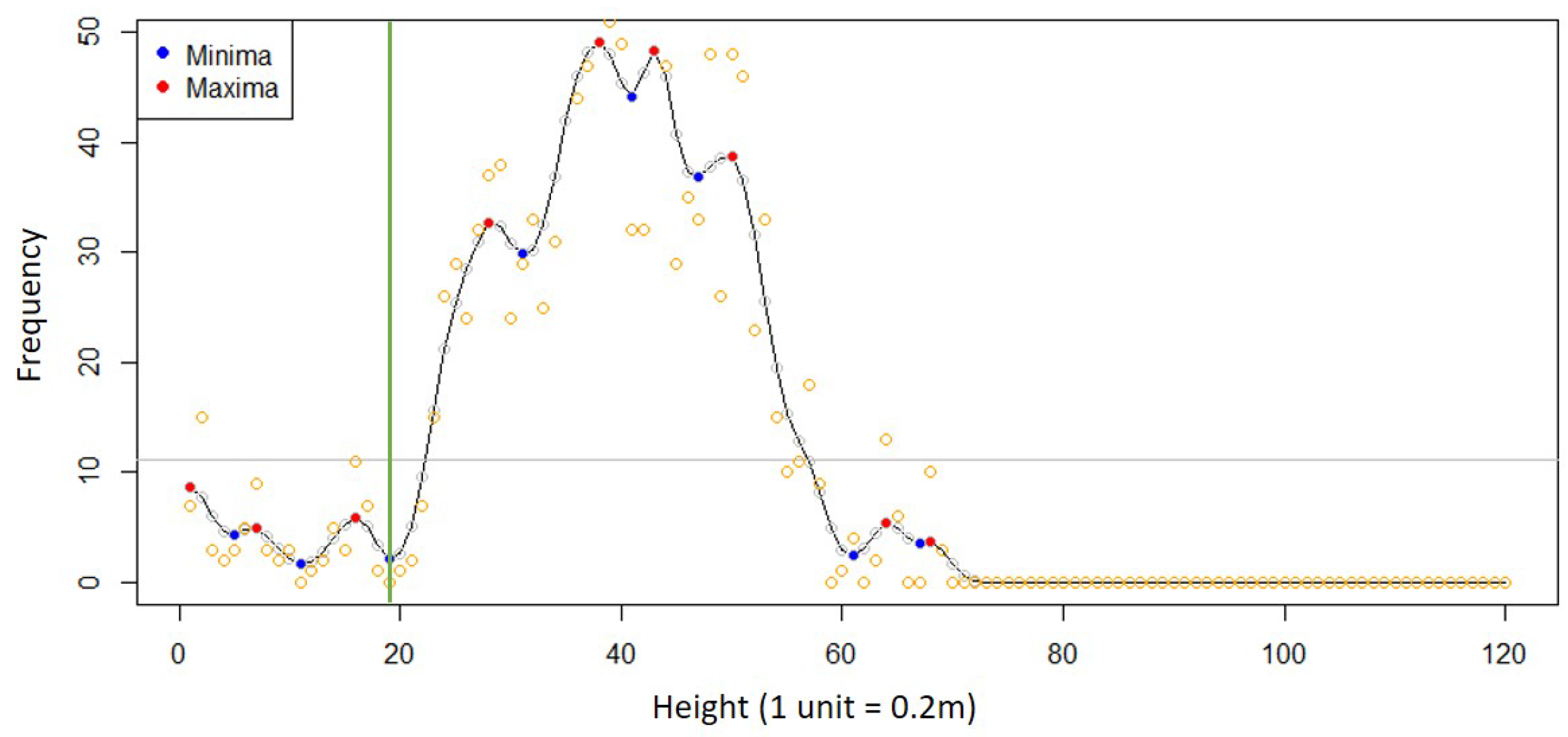
After point cloud voxelization, voxels that fell outside the actual plot edges were removed. In case a vertical voxel stack over a 10 m cell (hereafter referred to as bin) lacked point frequency information (i.e., only one or none of the bin voxels contained points), they were retained from further analysis. Point frequencies of each bin were smoothed using the Nadaraya-Watson kernel regression method [34] (Figure 5: grey points connected by line) and local minima and maxima were subsequently detected (Figure 5).
CBH for each bin was defined at the height of the local minimum followed by the first significant local maximum (i.e., above average point frequency of the bin) (Figure 5: vertical green line). Finally, the plot-level CBH was calculated as the average of all bin CBH values.
3.3. Plot-Level Regression Analysis
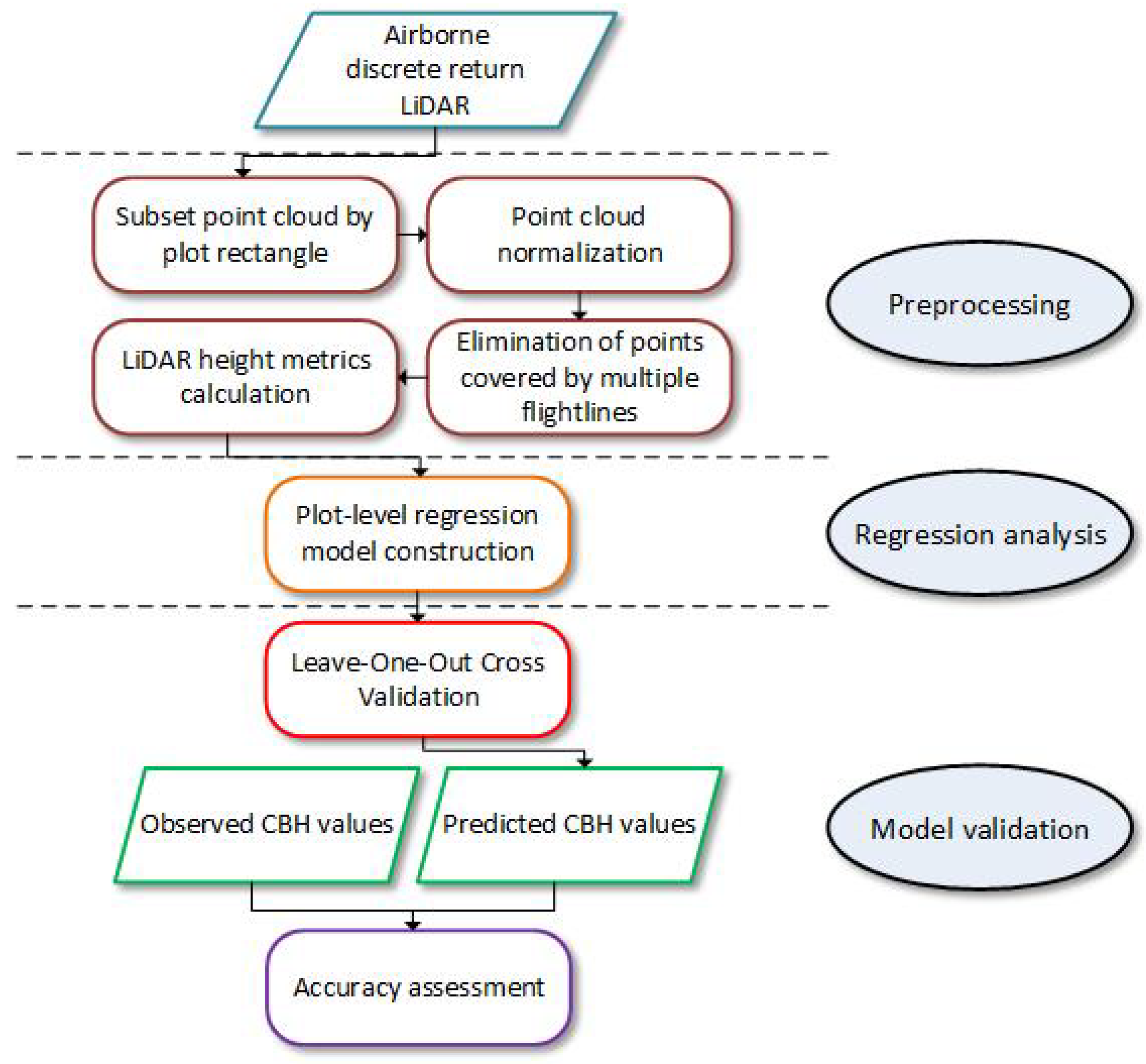
Similarly to the voxel-based method, LiDAR data were preprocessed prior to regression analysis (Figure 6). First, the point cloud covering each plot area was extracted and normalized by kNN-IDW method. Points covered by multiple flightlines were subsequently eliminated and a suite of LiDAR structural descriptive statistics (hereafter referred to as metrics) was calculated using the LAStools software and rLiDAR package implemented in R. In particular, height-normalized last-of-many and single (ls), last-of-many (l), first-of-many and single (fs), first-of-many (f) and total returns were extracted from the region of each plot. 47 plot-level metrics were computed from each extracted point cloud (i.e., ls, l, fs, f, all) including percentiles and bincentiles at relative heights as well as height value statistics (Table 2).
Linear regression was subsequently used for the construction of a plot-level CBH prediction model. The LiDAR metrics were initially examined for their correlation with field CBH individually and the most highly correlated ones were considered as candidate predictors in the model. Following the general rule of thumb of ten samples per one predictor [35], we tried not to exceed three predictors in the model and simultaneously minimize RMSE and avoid overfitting. The incorporation of additional predictors would increase model’s complexity and the risk of overfitting, due to the limited number of sample plots. The selection of the optimal predictor variables and appropriate transformations was manually performed trying to achieve maximum fit between the observed and estimated CBH values.
Once the predictive model was constructed, it was applied to the entire forest area in order to generate the respective CBH map.
3.4. Validation
Four standard goodness-of-fit metrics, namely coefficient of determination () (Equation (1)), Root Mean Square Error (RMSE) (Equation (2)), relative Root Mean Square Error (rRMSE) (Equation (3)) and relative bias (rbias) (Equation (4)), were calculated for the validation of the CBH estimated by means of the voxel-based approach (Section 3.2).
where is the observed CBH for plot i, is the predicted CBH for plot i, is the mean observed CBH and n the number of observations (i.e., number of sample plots).
The performance of the developed plot-level regression model was evaluated through Leave-One-Out Cross Validation (LOOCV) analysis. The predicted CBH values were assessed for their accuracy using the afore-described statistical measures (Equations (1)–(4)). Due to the log-transformation of the response variable in the model, the residual variance () (Equation (5)) was calculated in order to perform bias correction (Equation (6)) and calculate the actual estimated CBH values in the original scale.
where is the residual variance, is the observed CBH for plot i, is the predicted CBH for plot i, is the actual predicted CBH value in the original scale for plot i and n the number of observations (i.e., number of sample plots).
4. Results
4.1. Voxel-Based Approach Results
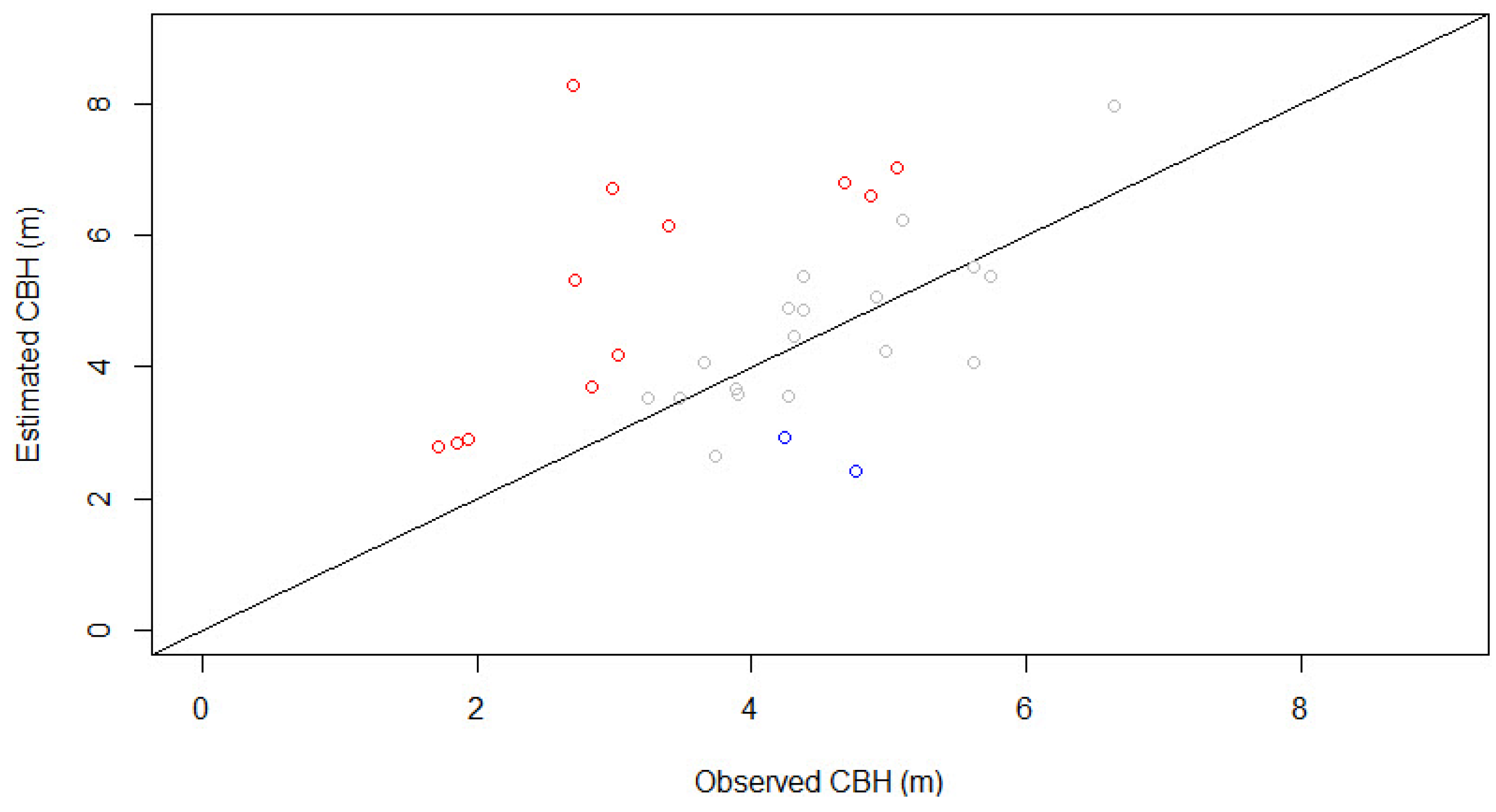
Table 3 and Figure 7 present a statistical summary and comparison of the field measured and voxel-based estimated CBH respectively. The results showcase a significant overestimation (i.e., error %) in 12 of the sample plots (red points of Figure 7) and underestimation in two of them (blue points in Figure 7). Overall, no correlation was found between the field measured and predicted CBH values. In particular, , , and were , m, and respectively.
4.2. Plot-Level Linear Regression Model
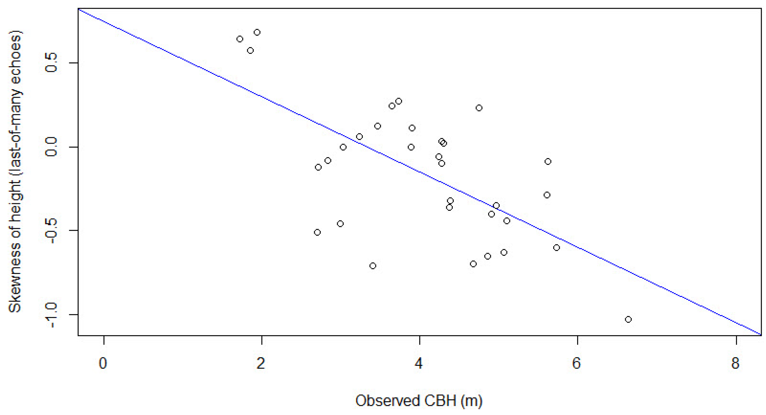
The examination of the individual LiDAR metrics correlation with the field measured CBH revealed that the skewness of height for the last-of-many echoes was the most important predictor with (Figure 8).
The final model (Equation (7)) developed via regression analysis includes three independent variables and five of the computed LiDAR metrics (Table 2), namely skewness of height (), 85th and 99th height percentiles ( and respectively), 50th bincentile () and 90th bincentile (b90). Metrics with l suffices refer to the last-of many echoes while no presence of suffix means that the metric was calculated including the entire point cloud.
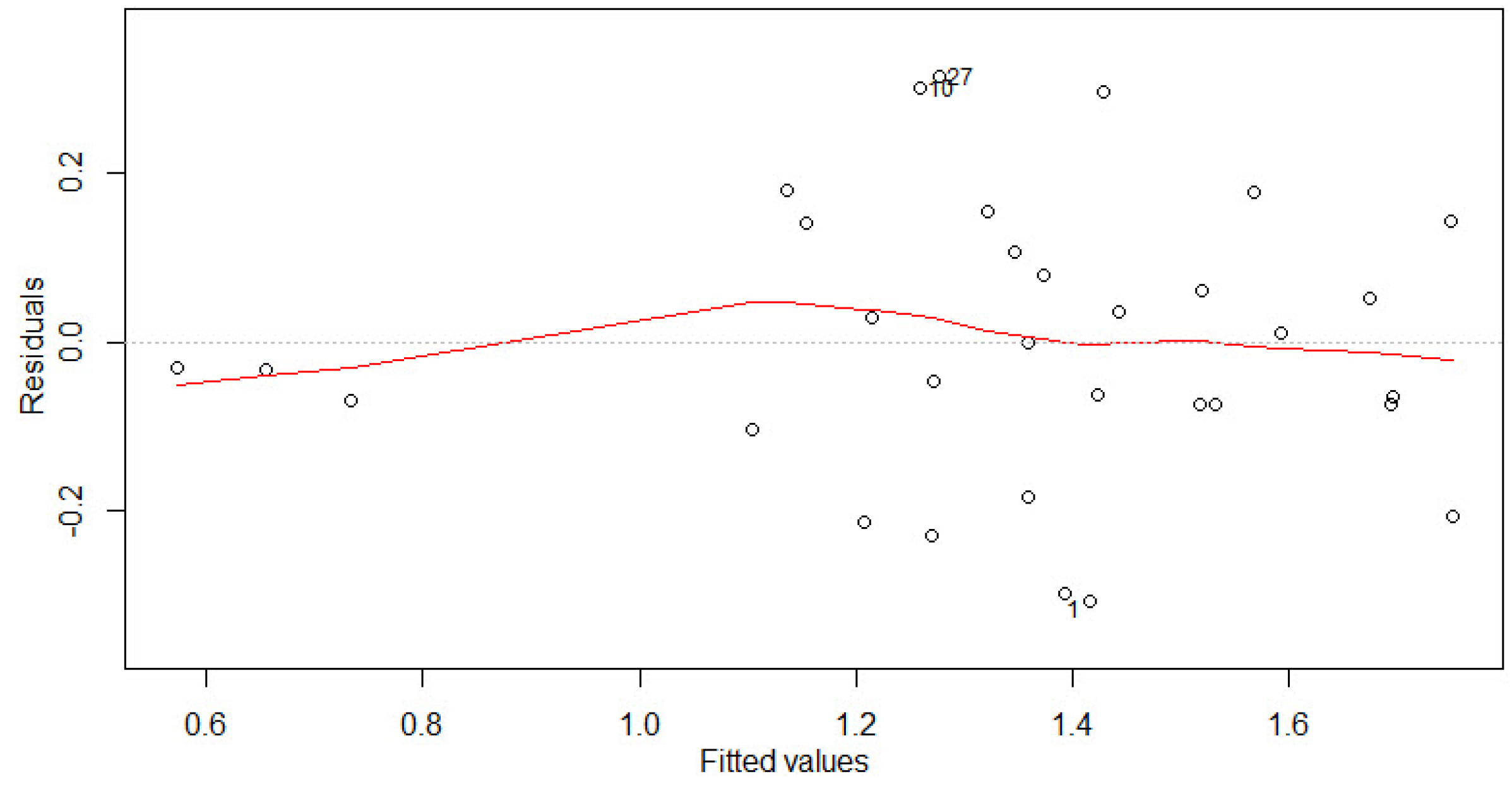
The fitted model has an , , and of 0.75, 0.66 m, 16.38% and respectively. The statistical measures derived by the estimated CBH values after the LOOCV process are , m, and . A scatterplot of the observed vs. the predicted CBH values and the residuals plot are presented in Figure 9 and Figure 10 respectively.
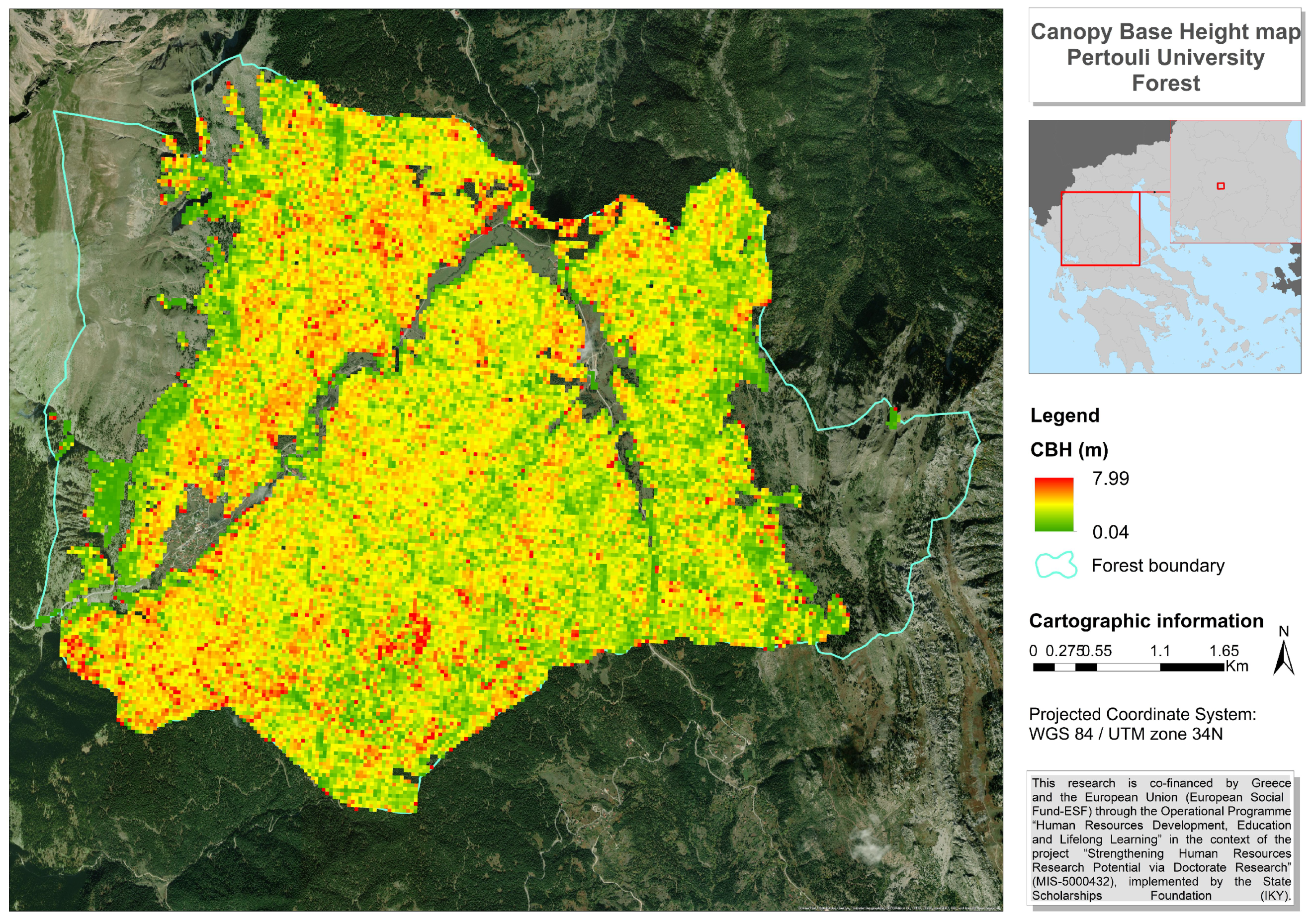
Figure 11 illustrates the CBH map produced at a spatial resolution of 32 m for the study area by employing the developed model to the entire LiDAR point cloud.
5. Discussion
In this study, plot-level CBH was estimated for a dense uneven-aged structured forest over complex terrain using high-density LiDAR data. The implemented estimation methods, namely the voxel-based and regression analysis approach, led to highly variate results. The former method failed to provide accurate CBH predictions for a significant number of sample plots. On the contrary, regression analysis resulted in the development of a prediction model with 3 independent variables which led to considerably more accurate predictions. The results of both methods are discussed in detail in Section 5.1, Section 5.2 and Section 5.3.
5.1. Voxel-Based Estimation
As reported in Section 4.1, a lack of correlation between measured and estimated CBH values was found (i.e., ). 18 of the 32 plots were accurately estimated in contrast to the remaining 14 plots which presented estimation errors higher than 30%. The latter plots were thoroughly examined in terms of vegetation structure and topography—information obtained from the field work—and visual inspection of the LiDAR point cloud was additionally performed.
Major underestimation errors occurred in two of the plots (i.e., plots 10 and 11 of Table 1). Field records of the specific areas indicated the presence of understorey vegetation which is close or overlapping with the dominant layers. These understorey conditions were confirmed by visual examination of the respective LiDAR point clouds. Figure 12 illustrates the vertical profile of plot 10 where CBH was severely underestimated (error 49.26%). In this case, the high understorey vegetation creates a continuous vertical point distribution extending from nearly the ground up to the top of the canopy. As a result, no vertical gaps are created which would facilitate the discrimination of the CBH. Although we agree with other authors stating that understorey vegetation renders the vertical LiDAR profile too noisy [3], the discrimination and elimination of understorey vegetation from the point cloud would not be able to benefit the results accuracy (related details in Section 3.2), at least within the scope of the current context.
Considerable overestimation errors were encountered in 12 of the 14 miscalculated plot-level CBH values. The majority of these plots are characterized by a low CBH (<3 m) compared to those of higher CBH values. In fact, eight out of the 12 plots have a reference plot-level CBH ranging between 1.72 m and 2.99 m respectively. A more detailed analysis of the total number of even slightly overestimated plots revealed a positive correlation between the estimation error and the distance of the reference CBH from the average canopy height. This type of correlation implies that the point cloud is not sufficiently dense in the lower parts of the canopy. The low number of returns from these layers is a strong indicator of the insufficient penetrating characteristics of the laser pulse at the specific areas which impacts the ability to accurately estimate the CBH or any other forest structural parameter related to the understorey vegetation.
A variety of potential factors may influence laser pulse penetration through the canopy including sensor settings, flight conditions, season of data acquisition and canopy characteristics. The pulse repetition frequency (PRF) (i.e., number of emitted pulses per second) is an important factor affecting pulse penetration and has been examined—among others—by Chasmer et al., (2006) and Massaro et al., (2012) [36,37]. Both studies reported that pulses of lower frequencies have greater penetration capabilities while Chasmer et al., (2012) stated that PRF has the opposite effect in stands with significant understorey presence. Scan angle also constitutes a substantial influence factor. According to Qin et al., (2017), foliage vertical profiles aren’t necessarily represented best with shallow scan angles but with 20 instead since increased angle leads to enhanced return energy from the lower canopy [38]. Weather considerably affects penetration rates as well, as reported by Hsu et al., (2015). The study indicates that pulse penetration decreases when wet and/or humid conditions are present because infrared light does not penetrate water vapor. Other studies have reported that a low pulse penetration rate can further be attributed to increased canopy height, density and cover levels [39,40].
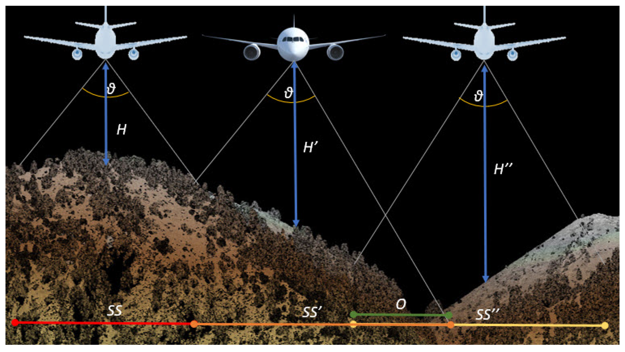
In case of CBH estimation by means of vertical profile analysis, a uniform return density is essential as it prevents the acquisition of decreased number of returns in some parts of the obtained LiDAR data. It can be achieved by maintaining a constant aboveground flying height which however becomes challenging over steep mountainous terrain especially during windy days [41] (Figure 13). Additionally, steep slopes may impact the laser scanning swath leading to a similar point density variation. Plots located on hilly terrain may partially lack points from one side due to the resulting change in scanning swath between adjacent flightlines (Figure 13). The number of echoes from the low part of the canopy is also substantially affected by crown length which variates among different tree species. For example, mature spruce trees are generally characterized by longer crown lengths compared to pines which may result in more accurate CBH estimation of the latter [42].
Although each of the above-mentioned factors can explain CBH miscalculations, it is very challenging to define particular reasons. The results’ examination revealed that the lack of correlation between field measured and estimated CBH values may be simultaneously attributed to multiple causes. While we could not explore the effect of certain components on the estimation accuracy of our study (e.g., effects of difference in scanning angle or PRF), we examined the factors that present variation among the sample plot areas. A prominent example is the effect of canopy height, cover and slope on estimation accuracy. Although the individual correlation of these forest parameters with CBH accuracy was rather low (i.e., of , and 0.16 for canopy cover, slope and mean canopy height respectively), their interactive impact was observed. More specifically, the negative effect of high canopy (i.e., increased crown length) on the quantity of low points and the subsequent estimation accuracy was reduced in cases where canopy cover and slope were relatively low compared to other areas with high cover and steep slopes. The same applies to areas of intense relief but lower canopy height and cover.
Taking all under consideration, the voxel-based analysis approach applied in this study was not able to deliver accurate CBH estimations over a forested land which is highly diverse and complex in terms of forest structure and terrain.
5.2. Regression Analysis
Three statistically significant predictors were used in the developed predictive model (Equation (7)) including five LiDAR-retrieved metrics, namely the , , , and (Table 2). All were calculated using the last-of-many returns of the point cloud except for the which was derived by the total number of echoes. The fact that metrics of last-of-many returns were mostly chosen as predictors indicates the direct interaction of LiDAR with the lower part of the canopy while the use of the entire point cloud shows an indirect CBH estimation through its association with the canopy conditions.
Skewness and percentiles of height have been successfully used in the literature for describing CBH in various vegetation and topography conditions such as pine plantations in SW Spain, forested watershed and mountain pine stands at very high elevations in the US [4,15,21,43]. In our study, was the variable mostly correlated (i.e., negative relationship) with the reference data (Figure 8) as it is a measure of the height distribution shape from which CBH is derived. The use of the percentiles of last-of-many returns is a logical selection for describing CBH since these metrics describe the bottom of the canopy better than percentiles of other echo types. In fact, visual examination of the LiDAR data revealed that ground returns were seldom obtained from beneath the canopy but mostly from canopy openings. Thus, last-of-many echoes were dominated by reflection from within the canopy, including both bottom and top layers.
Due to the variance in pulse penetration depth along the study area (explained in Section 5.1), the exclusive use of height percentiles was considered insufficient for CBH prediction in our research. Height bincentile metrics were found to complement this insufficiency since they depict the percentage of points below an indicated height (e.g., 85th bincentile = % points below the 85% of the point cloud’s maximum height). In other words, height bincentiles (i.e., and ) were used as an indirect proxy of the pulse penetration depth through the canopy. A higher bincentile value means that more returns are registered below a certain elevation, thus the pulse has penetrated deeper in the canopy compared to an area characterized by a lower bincentile value. In fact, canopy cover and mean canopy height, which influence the pulse penetration depth (described in Section 5.1), were calculated from the LiDAR data and individually examined for their correlation with the field-measured CBH. The results showcased an R of 0.11 and 0.17 for the canopy cover and mean height respectively. To this end, the individual use of height and density related LiDAR metrics in the prediction model would lead to a rather lower predictive performance.
While it is difficult to interpret the use of sums and interactions between the metrics employed in the produced regression model, the combination of a percentile and a bincentile metric in one predictive variable seems logical since, as mentioned above, percentile metrics could not encompass the high variability of the forest in terms of vegetation density and topography. The logarithmic transformation of CBH was used to deal with variance instability, mitigating heteroscedasticity of the residual plot.
The employment of the afore-described LiDAR metrics led to the construction of a regression model (Equation (7)), which—according to the cross validation results reported in Section 4.2—can reliably predict plot-level CBH. In particular, the model can explain 61% of the variability in the linearized space derived from the variables transformations. The models fit to compare the predicted with the reference data is similar to the hypothetical 1:1 relationship (Figure 9). Plot-level CBH was predicted by the model with 18.19% of and a negative of %.
Significant caution is required when directly comparing regression results derived from different studies due to differences in forest types, LiDAR sensors and flight specifications, topography, response variables and employed transformations in the regression model. Nevertheless, it is worth noting that RMSE in our study may be higher compared to other reported earlier. The reason may possibly encompass many of the above mentioned factors but also may just be related to the generally lower reference CBH values of our study area.
The predictive model was applied to the LiDAR point cloud covering the entire study area generating a CBH map (Figure 11), which provides spatial plot-level CBH information at a resolution of 32m. Visual examination of the map CBH values along with aerial photo-interpretation revealed evident estimation errors in limited areas of the forest. CBH values approximating zero were calculated either over forest openings covered by few trees or very sparse stands while extremely high values—eliminated from the final CBH map—were located at the forest boundaries due to edge effects reported in other relevant studies as well [18,19,21,23,38]. This is an expected outcome since the model was constructed with the use of sample plots located exclusively over dense forested land with no sparsely wooded areas or forest openings involved.
5.3. Methods Comparison and Limitations
An overall analysis of the results (Section 4.1 and Section 4.2) revealed that regression-based estimation provides more reliable CBH predictions in structurally complex forests over variant topographic conditions. In fact, the advantages of the voxel-based approach over the regression method (described in Section 1) proved unable to compensate for the heterogeneity in structure and terrain characterizing the study area.
Despite certain limitations presented by the regression analysis method (described in Section 1), the results showcased that it is less sensitive to understorey conditions compared to the voxel-based method. This is of utmost importance in our study area where the understorey (where present) may overlap with the canopy leading to absence of vertical gaps and a subsequent difficulty in eliminating the understorey points, which could not be overcome in the context of our work. On the contrary, structural point cloud analysis based on voxels resulted in substantial underestimation errors in plots with intense presence of understorey growth.
Being sensitive to any structural characteristics of the LiDAR point cloud, the inconsistent accuracy results derived by the voxel-based estimation method reflect the respective deviation in terms of forest and terrain contexts which enhanced point density variation in the lower parts of the canopy. Nevertheless, the method gave accurate estimates in the majority of sample plots where CBH was not low (i.e., >3 m), indicating that accurate estimation could be achieved for forest species of generally higher CBH (e.g., mature pines).
Although the present study has reached its aims, there were some limitations affecting both methods. First, field measurement accuracy is essential for acquiring reliable predictions especially in regression analysis approach. In addition, uncertainties in GPS measurements were present. Although the GPS horizontal accuracy was just 3 m, the possible geographic misplacement of the rectangular plots may greatly influence the estimation outcomes. This problem has been probably alleviated by the selection of large sample plots (1000 m) which may have mitigated a possible inherent variability and the subsequent variation in predictions derived especially by the regression-based method. Moreover, the results of the study indicate that both employed methods require very high-density LiDAR in order to better represent vegetation structure from the lower part of the canopy, at least within the existing forest contexts. The small number of sample plots constitutes an additional limitation of this work as most related studies recommend the use of more than 40 samples in regression analysis implementations [44].
Finally, the predictive model developed in this study should not be considered as transferable to other forest ecosystems with differences in species composition, phenology and topography characteristics. Although performing well in our study area, a new model should be developed for a different area using new reference CBH values since variation in LiDAR data acquisition specifications, vegetation characteristics and/or topography negatively influences the model’s transferability to other forested areas.
6. Conclusions
The present work focused on the CBH estimation of an uneven-aged structured forest located over complex terrain. Two widely used methods, namely the voxel-based approach and regression analysis, were applied and accordingly evaluated. The results showcased a substantial outperformance of the regression-based estimation method. More specifically:
- The voxel-based method implementation led to CBH prediction with no adequate correlation with the reference data (). In most of the plots CBH was overestimated () with the reaching .
- Regression analysis resulted in a predictive model of high performance, given the heterogeneity of the study area. Cross-validation revealed an and of and respectively and a limited overestimation trend ().
- The voxel-based approach could not successfully respond to variations characterizing the structural and topographic conditions within the forest. Its’ estimation accuracy is determined by the LiDAR pulses penetration properties, thus highly susceptible to the quantity of points from low canopy parts, which are used to define CBH.
- The use of LiDAR-retrieved metrics in regression analysis compensated for the variance in vegetation structure and terrain across the study area.
- The developed predictive model can be used to generate a CBH map over the entire study area (Figure 11) for direct employment by forest and fire managers.
Given the above mentioned conclusions, further research requires the investigation of the potential of full-waveform or discrete-return LiDAR data of higher point density to estimate plot-level CBH over the same study area, which could not be achieved in the framework of this research due to legal restrictions. Such LiDAR data would probably provide more structural information from the low parts of the canopy resulting in more reliable CBH predictions. Moreover, the probable acquisition of spaceborne LiDAR data would provide a cost-effective alternative and the examination of their potential capability to accurately predict CBH in complex forests would be of high interest and importance.
Author Contributions
Conceptualization, A.S., I.Z.G. and L.K.; methodology, A.S. and L.K.; software, A.S. and D.S.; validation, A.S. and N.G.; formal analysis, A.S., D.S. and N.G.; investigation, A.S.; resources, I.Z.G.; data curation, A.S.; writing—original draft preparation, A.S.; writing—review and editing, A.S., I.Z.G. and L.K.; visualization, A.S.; supervision, I.Z.G. and L.K.; project administration, I.Z.G. All authors have read and agreed to the published version of the manuscript.
Funding
This research is co-financed by Greece and the European Union (European Social Fund-ESF) through the Operational Programme “Human Resources Development, Education and Lifelong Learning” in the context of the project “Strengthening Human Resources Research Potential via Doctorate Research” (MIS-5000432), implemented by the State Scholarships Foundation (IKY).
Conflicts of Interest
The authors declare no conflict of interest.
References
- Luo, L.; Zhai, Q.; Su, Y.; Ma, Q.; Kelly, M.; Guo, Q. Simple method for direct crown base height estimation of individual conifer trees using airborne LiDAR data. Opt. Express 2018, 26, A562. [Google Scholar] [CrossRef] [PubMed]
- Xu, W.; Su, Z.; Feng, Z.; Xu, H.; Jiao, Y.; Yan, F. Comparison of conventional measurement and LiDAR-based measurement for crown structures. Comput. Electron. Agric. 2013, 98, 242–251. [Google Scholar] [CrossRef]
- Popescu, S.C.; Zhao, K. A voxel-based lidar method for estimating crown base height for deciduous and pine trees. Remote Sens. Environ. 2008, 112, 767–781. [Google Scholar] [CrossRef]
- Hermosilla, T.; Ruiz, L.A.; Kazakova, A.N.; Coops, N.C.; Moskal, L.M. Estimation of forest structure and canopy fuel parameters from small-footprint full-waveform LiDAR data. Int. J. Wildland Fire 2014, 23, 224. [Google Scholar] [CrossRef] [Green Version]
- Cruz, M.G.; Alexander, M.E.; Wakimoto, R.H. Assessing canopy fuel stratum characteristics in crown fire prone fuel types of western North America. Int. J. Wildland Fire 2003, 12, 39. [Google Scholar] [CrossRef] [Green Version]
- Bianchi, S.; Siipilehto, J.; Hynynen, J. How structural diversity affects Norway spruce crown characteristics. For. Ecol. Manag. 2020, 461, 117932. [Google Scholar] [CrossRef]
- Kara, F.; Topaçoğlu, O. Influence of stand density and canopy structure on the germination and growth of Scots pine (Pinus sylvestris L.) seedlings. Environ. Monit. Assess. 2018, 190, 749. [Google Scholar] [CrossRef]
- Dobbertin, M. Tree growth as indicator of tree vitality and of tree reaction to environmental stress: A review. Eur. J. For. Res. 2005, 124, 319–333. [Google Scholar] [CrossRef]
- Pyörälä, J.; Saarinen, N.; Kankare, V.; Coops, N.; Liang, X.; Wang, Y.; Holopainen, M.; Hyyppä, J.; Vastaranta, M. Variability of wood properties using airborne and terrestrial laser scanning. Remote Sens. Environ. 2019, 235, 111474. [Google Scholar] [CrossRef]
- Jia, W.; Chen, D. Nonlinear mixed-effects height to crown base and crown length dynamic models using the branch mortality technique for a Korean larch (Larix olgensis) plantations in northeast China. J. For. Res. 2019, 30, 2095–2109. [Google Scholar] [CrossRef]
- Zarnoch, S.J.; Bechtold, W.A.; Stolte, K.W. Using crown condition variables as indicators of forest health. Can. J. For. Res. 2004, 34, 1057–1070. [Google Scholar] [CrossRef]
- Finney, M.A. FARSITE, Fire Area Simulator–Model Development and Evaluation; Number 4; US Department of Agriculture, Forest Service, Rocky Mountain Research Station: Fort Collins, CO, USA, 1998.
- Finney, M.A. An overview of FlamMap fire modeling capabilities. In Fuels Management-How to Measure Success, Proceedings of the RMRS-P-41 Conference, Portland, OR, USA, 28–30 March 2006; Patricia, L.A., Bret, W.B., Eds.; US Department of Agriculture, Forest Service, Rocky Mountain Research Station: Fort Collins, CO, USA, 2006; Volume 41, pp. 213–220. [Google Scholar]
- Andrews, P.L. BEHAVE: Fire Behavior Prediction and Fuel Modeling System: BURN Subsystem; US Department of Agriculture, Forest Service, Intermountain Research Station: Fort Collins, CO, USA, 1986; Volume 194.
- Riaño, D.; Meier, E.; Allgöwer, B.; Chuvieco, E.; Ustin, S.L. Modeling airborne laser scanning data for the spatial generation of critical forest parameters in fire behavior modeling. Remote Sens. Environ. 2003, 86, 177–186. [Google Scholar] [CrossRef]
- Engelstad, P.S.; Falkowski, M.; Wolter, P.; Poznanovic, A.; Johnson, P. Estimating Canopy Fuel Attributes from Low-Density LiDAR. Fire 2019, 2, 38. [Google Scholar] [CrossRef] [Green Version]
- Luo, S.; Chen, J.M.; Wang, C.; Xi, X.; Zeng, H.; Peng, D.; Li, D. Effects of LiDAR point density, sampling size and height threshold on estimation accuracy of crop biophysical parameters. Opt. Express 2016, 24, 11578–11593. [Google Scholar] [CrossRef] [PubMed]
- Sumnall, M.; Peduzzi, A.; Fox, T.R.; Wynne, R.H.; Thomas, V.A. Analysis of a lidar voxel-derived vertical profile at the plot and individual tree scales for the estimation of forest canopy layer characteristics. Int. J. Remote. Sens. 2016, 37, 2653–2681. [Google Scholar] [CrossRef]
- Andersen, H.E.; McGaughey, R.J.; Reutebuch, S.E. Estimating forest canopy fuel parameters using LIDAR data. Remote Sens. Environ. 2005, 94, 441–449. [Google Scholar] [CrossRef]
- Erdody, T.L.; Moskal, L.M. Fusion of LiDAR and imagery for estimating forest canopy fuels. Remote Sens. Environ. 2010, 114, 725–737. [Google Scholar] [CrossRef]
- González-Ferreiro, E.; Diéguez-Aranda, U.; Crecente-Campo, F.; Barreiro-Fernández, L.; Miranda, D.; Castedo-Dorado, F. Modelling canopy fuel variables for Pinus radiata D. Don in NW Spain with low-density LiDAR data. Int. J. Wildland Fire 2014, 23, 350. [Google Scholar] [CrossRef]
- Maguya, A.; Tegel, K.; Junttila, V.; Kauranne, T.; Korhonen, M.; Burns, J.; Leppanen, V.; Sanz, B. Moving Voxel Method for Estimating Canopy Base Height from Airborne Laser Scanner Data. Remote Sens. 2015, 7, 8950–8972. [Google Scholar] [CrossRef] [Green Version]
- Karjalainen, T.; Korhonen, L.; Packalen, P.; Maltamo, M. The transferability of airborne laser scanning based tree-level models between different inventory areas. Can. J. For. Res. 2019, 49, 228–236. [Google Scholar] [CrossRef] [Green Version]
- Næsset, E. Predicting forest stand characteristics with airborne scanning laser using a practical two-stage procedure and field data. Remote Sens. Environ. 2002, 80, 88–99. [Google Scholar] [CrossRef]
- Botequim, B.; Fernandes, P.M.; Borges, J.G.; González-Ferreiro, E.; Guerra-Hernández, J. Improving silvicultural practices for Mediterranean forests through fire behaviour modelling using LiDAR-derived canopy fuel characteristics. Int. J. Wildland Fire 2019, 28, 823–839. [Google Scholar] [CrossRef]
- Kelly, M.; Su, Y.; Di Tommaso, S.; Fry, D.L.; Collins, B.M.; Stephens, S.L.; Guo, Q. Impact of Error in Lidar-Derived Canopy Height and Canopy Base Height on Modeled Wildfire Behavior in the Sierra Nevada, California, USA. Remote Sens. 2017, 10, 10. [Google Scholar] [CrossRef] [Green Version]
- Hevia, A.; Álvarez González, J.G.; Ruiz-Fernández, E.; Prendes, C.; Ruiz-González, A.D.; Majada, J.; González-Ferreiro, E. Estimación de variables de combustible de copa y de masa, caracterizando el efecto de las claras en su estructura usando LiDAR aerotransportado. Rev. Teledetección 2016, 41. [Google Scholar] [CrossRef] [Green Version]
- Vauhkonen, J. Estimating crown base height for Scots pine by means of the 3D geometry of airborne laser scanning data. Int. J. Remote Sens. 2010, 31, 1213–1226. [Google Scholar] [CrossRef]
- Dean, T.J.; Cao, Q.V.; Roberts, S.D.; Evans, D.L. Measuring heights to crown base and crown median with LiDAR in a mature, even-aged loblolly pine stand. For. Ecol. Manag. 2009, 257, 126–133. [Google Scholar] [CrossRef]
- Sumnall, M.; Fox, T.R.; Wynne, R.H.; Thomas, V.A. Mapping the height and spatial cover of features beneath the forest canopy at small-scales using airborne scanning discrete return Lidar. ISPRS J. Photogramm. Remote Sens. 2017, 133, 186–200. [Google Scholar] [CrossRef]
- Hsu, W.C.; Shih, P.T.Y.; Chang, H.C.; Liu, J.K. A Study on Factors Affecting Airborne LiDAR Penetration. Terr. Atmos. Ocean. Sci. 2015, 26, 241. [Google Scholar] [CrossRef]
- Maltamo, M.; Karjalainen, T.; Repola, J.; Vauhkonen, J. Incorporating tree- and stand-level information on crown base height into multivariate forest management inventories based on airborne laser scanning. Silva Fenn. 2018, 52, 10006. [Google Scholar] [CrossRef]
- Laar, A.V.; Akça, A. Forest Mensuration, 2nd ed.; completely rev. and supplemented ed.; Number Volume 13 in Managing Forest Ecosystems; Springer: Dordrecht, The Netherlands, 2007; OCLC: 255827796. [Google Scholar]
- Nadaraya, E.A. On estimating regression. Theory Probab. Its Appl. 1964, 9, 141–142. [Google Scholar] [CrossRef]
- Miller, D.E.; Kunce, J.T. Prediction and Statistical Overkill Revisited. Meas. Eval. Guid. 1973, 6, 157–163. [Google Scholar] [CrossRef]
- Chasmer, L.; Hopkinson, C.; Smith, B.; Treitz, P. Examining the Influence of Changing Laser Pulse Repetition Frequencies on Conifer Forest Canopy Returns. Photogramm. Eng. Remote Sens. 2006, 72, 1359–1367. [Google Scholar] [CrossRef] [Green Version]
- Massaro, R.; Zinnert, J.; Anderson, J.; Edwards, J.; Crawford, E.; Young, D. Lidar Flecks: Modeling the Influence of Canopy Type on Tactical Foliage Penetration by Airborne, Active Sensor Platforms. In Proceedings of the SPIE 8360, Airborne Intelligence, Surveillance, Reconnaissance (ISR) Systems and Applications IX, Baltimore, MD, USA, 3 May 2012; Volume 8360, p. 836008. [Google Scholar] [CrossRef]
- Qin, H.; Wang, C.; Xi, X.; Tian, J.; Zhou, G. Simulating the Effects of the Airborne Lidar Scanning Angle, Flying Altitude, and Pulse Density for Forest Foliage Profile Retrieval. Appl. Sci. 2017, 7, 712. [Google Scholar] [CrossRef] [Green Version]
- Takahashi, T.; Yamamoto, K.; Miyachi, Y.; Senda, Y.; Tsuzuku, M. The penetration rate of laser pulses transmitted from a small-footprint airborne LiDAR: A case study in closed canopy, middle-aged pure sugi (Cryptomeria japonica D. Don) and hinoki cypress (Chamaecyparis obtusa Sieb. et Zucc.) stands in Japan. J. For. Res. 2006, 11, 117–123. [Google Scholar] [CrossRef]
- Wieser, M.; Hollaus, M.; Mandlburger, G.; Glira, P.; Pfeifer, N. ULS LiDAR supported analyses of laser beam penetration from different ALS systems into vegetation. ISPRS Ann. Photogramm. Remote Sens. Spat. Inf. Sci. 2016, III-3, 233–239. [Google Scholar] [CrossRef]
- Gatziolis, D.; Andersen, H.E. A Guide to LIDAR Data Acquisition and Processing for the Forests of the Pacific Northwest; Technical Report PNW-GTR-768; U.S. Department of Agriculture, Forest Service, Pacific Northwest Research Station: Portland, OR, USA, 2008. [CrossRef]
- Holmgren, J.; Persson, A. Identifying species of individual trees using airborne laser scanner. Remote Sens. Environ. 2004, 90, 415–423. [Google Scholar] [CrossRef]
- Bright, B.; Hudak, A.; Meddens, A.; Hawbaker, T.; Briggs, J.; Kennedy, R. Prediction of Forest Canopy and Surface Fuels from Lidar and Satellite Time Series Data in a Bark Beetle-Affected Forest. Forests 2017, 8, 322. [Google Scholar] [CrossRef] [Green Version]
- Gobakken, T.; Korhonen, L.; Næsset, E. Laser-assisted selection of field plots for an area-based forest inventory. Silva Fenn. 2013, 47, 1–20. [Google Scholar] [CrossRef] [Green Version]
Figure 1.
Study area map including vegetation cover distribution (source: forest management plan of the year 2018) and sample plots location.
Figure 1.
Study area map including vegetation cover distribution (source: forest management plan of the year 2018) and sample plots location.

Figure 2.
A vertical cross section of plot 29 (Table 1). The horizontal dashed line represents the plot-level CBH measured on the field.
Figure 2.
A vertical cross section of plot 29 (Table 1). The horizontal dashed line represents the plot-level CBH measured on the field.

Figure 3.
Schematic workflow of the voxel-based method for estimating canopy base height (CBH).

Figure 4.
Example of a tree, only a part of which was extracted due to its’ location on the plot’s corner. (a) an illustration of the vertical cross section of the tree emphasizing the actual CBH and the one possibly estimated in case the tree points outside the plot’s border were not included in the analysis. (b) Vertical view of the tree showing the sides at which the tree was cut (i.e., upper and left side).

Figure 5.
A vertical point frequency distribution (orange points) graph of one bin (i.e., voxels over a 10 m resolution cell). X axis is the point frequency of the voxels and Y axis is the vertical order of the voxels starting from the ground (i.e., voxel with value 1 presents the point frequency between 0–0.2 m height etc.). The points in grey color connected by the black line represent the smoothed frequency values. Blue and red colored points refer to the detected local minima and maxima respectively. The horizontal grey line stands for the average point frequency of the entire bin and the vertical green line shows the estimated CBH (i.e., the height of the voxel, the point frequency of which is the local minima before the first significant local maxima).

Figure 6.
Schematic workflow for the regression-based estimation of canopy base height (CBH).

Figure 7.
Comparison of measured CBH with the one estimated by the voxel-based method. Overestimated CBH values with error higher than 30% are presented with red color and underestimated with blue.
Figure 7.
Comparison of measured CBH with the one estimated by the voxel-based method. Overestimated CBH values with error higher than 30% are presented with red color and underestimated with blue.

Figure 8.
A scatterplot of the skewness of height for the last-of-many echoes vs. the field measured CBH values ().
Figure 8.
A scatterplot of the skewness of height for the last-of-many echoes vs. the field measured CBH values ().

Figure 9.
Comparison of the field measured and the predicted CBH values ().

Figure 10.
Residuals in the prediction of plot-level CBH using regression analysis.

Figure 11.
Canopy base height (CBH) map (32 m spatial resolution) produced for the Pertouli University Forest by applying the predictive regression model to the LiDAR point cloud of the entire study area.
Figure 11.
Canopy base height (CBH) map (32 m spatial resolution) produced for the Pertouli University Forest by applying the predictive regression model to the LiDAR point cloud of the entire study area.

Figure 12.
Vertical cross sections of plot 10 which was significantly underestimated for its CBH. The presence of understorey vegetation being close or overlapping with the CBH can be visually observed.
Figure 12.
Vertical cross sections of plot 10 which was significantly underestimated for its CBH. The presence of understorey vegetation being close or overlapping with the CBH can be visually observed.

Figure 13.
Example of variations in aboveground flying height (H, , ) and scanning swath (, , ) over mountainous terrain ( = scan angle and O = overlapping area).
Figure 13.
Example of variations in aboveground flying height (H, , ) and scanning swath (, , ) over mountainous terrain ( = scan angle and O = overlapping area).


Table 1.
Summary of field plots used in this study.
| Plot ID | No. of Trees | CBH (m) | Elevation (m) | Slope (%) | Aspect |
|---|---|---|---|---|---|
| 1 | 53 | 3.03 | 1175 | 60–70 | NW |
| 2 | 56 | 3.89 | 1378 | 45–60 | E-SE |
| 3 | 45 | 3.73 | 1352 | 25–40 | W-NW |
| 4 | 65 | 3.65 | 1339 | 20–30 | E |
| 5 | 50 | 1.72 | 1335 | 10–20 | W-SW |
| 6 | 49 | 4.27 | 1285 | 40–50 | E-NE |
| 7 | 63 | 4.38 | 1304 | 30–40 | N |
| 8 | 113 | 4.97 | 1239 | 10–20 | NW |
| 9 | 50 | 3.90 | 1299 | 10–20 | W |
| 10 | 68 | 4.75 | 1254 | 40 | SE |
| 11 | 47 | 4.24 | 1190 | 10–30 | SW |
| 12 | 50 | 4.30 | 1177 | 40–60 | E-SE |
| 13 | 51 | 2.83 | 1170 | 40 | NW |
| 14 | 37 | 4.37 | 1194 | 20–40 | N-NE |
| 15 | 55 | 1.86 | 1220 | 40–60 | W-NW-N |
| 16 | 82 | 4.27 | 1182 | 10 | NE-SE |
| 17 | 47 | 3.24 | 1332 | 45–65 | SW |
| 18 | 64 | 5.10 | 1303 | 20–40 | S-SE |
| 19 | 39 | 6.63 | 1233 | 10–20 | E-SE |
| 20 | 57 | 5.73 | 1187 | 10–20 | SW |
| 21 | 38 | 1.94 | 1243 | 40–50 | SE |
| 22 | 51 | 4.86 | 1220 | 10–40 | NE-E-SE |
| 23 | 31 | 3.40 | 1201 | 10–30 | NE |
| 24 | 37 | 4.68 | 1266 | 40 | SE |
| 25 | 52 | 2.99 | 1220 | 30–40 | S |
| 26 | 74 | 5.06 | 1208 | 40–50 | E-SE |
| 27 | 45 | 4.91 | 1170 | 0–20 | E |
| 28 | 32 | 2.72 | 1179 | 10–40 | W-NW |
| 29 | 55 | 3.47 | 1186 | 10–20 | W-S |
| 30 | 118 | 5.61 | 1179 | 30–40 | S |
| 31 | 44 | 5.62 | 1222 | 20–40 | S |
| 32 | 21 | 2.70 | 1229 | 10–30 | N-NW-SE |
These attributes refer to the plot-level average values.
Table 2.
The LiDAR metrics used in this study for the construction of the plot-level CBH prediction regression model. The metrics refer to the pooled first-of-many and single echoes, pooled last-of-many and single echoes, last-of-many, first-of-many and total echoes.
Table 2.
The LiDAR metrics used in this study for the construction of the plot-level CBH prediction regression model. The metrics refer to the pooled first-of-many and single echoes, pooled last-of-many and single echoes, last-of-many, first-of-many and total echoes.
| LiDAR | Definition |
|---|---|
| p05, p10 … p95, p99 | Height percentiles |
| b05, b10 … b95, b99 | Height bincentiles |
| Hske | Skewness of height |
| Hkur | Kurtosis of height |
| CRR | Canopy relief ratio |
| Hmax | Maximum height value |
| Havg | Average height value |
| Hstd | Standard deviation of heights |
| Hqav | Average square height |
Table 3.
Statistical summary of the field measured and voxel-based estimated CBH.
| Statistical Measures | Measured CBH (m) | Estimated CBH (m) |
|---|---|---|
| Minimum | 1.72 | 2.41 |
| Maximum | 6.63 | 8.28 |
| Average | 4.03 | 4.73 |
| Standard deviation | 1.17 | 1.57 |
© 2020 by the authors. Licensee MDPI, Basel, Switzerland. This article is an open access article distributed under the terms and conditions of the Creative Commons Attribution (CC BY) license (http://creativecommons.org/licenses/by/4.0/).
Share and Cite
MDPI and ACS Style
Stefanidou, A.; Gitas, I.Z.; Korhonen, L.; Stavrakoudis, D.; Georgopoulos, N. LiDAR-Based Estimates of Canopy Base Height for a Dense Uneven-Aged Structured Forest. Remote Sens. 2020, 12, 1565. https://doi.org/10.3390/rs12101565
AMA Style
Stefanidou A, Gitas IZ, Korhonen L, Stavrakoudis D, Georgopoulos N. LiDAR-Based Estimates of Canopy Base Height for a Dense Uneven-Aged Structured Forest. Remote Sensing. 2020; 12(10):1565. https://doi.org/10.3390/rs12101565
Chicago/Turabian StyleStefanidou, Alexandra, Ioannis Z. Gitas, Lauri Korhonen, Dimitris Stavrakoudis, and Nikos Georgopoulos. 2020. "LiDAR-Based Estimates of Canopy Base Height for a Dense Uneven-Aged Structured Forest" Remote Sensing 12, no. 10: 1565. https://doi.org/10.3390/rs12101565
Note that from the first issue of 2016, this journal uses article numbers instead of page numbers. See further details here.